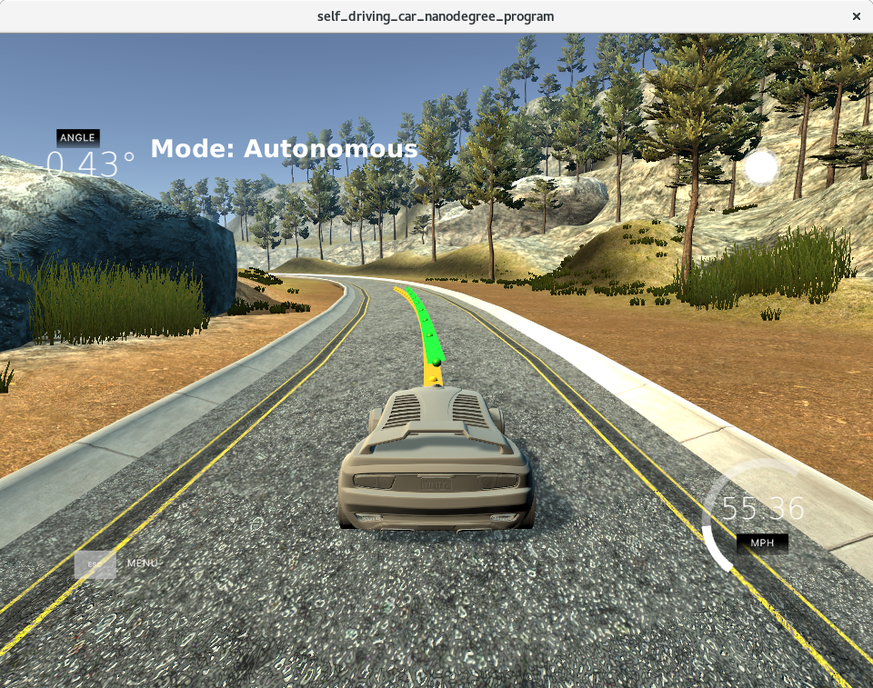
This project consists of a c++ implementation of a Model Predictive Control (MPC) to control the steering angle and the throttle acceleration of a car using the Udacity self driving simulator. The main goal of this project is to develop a c++ MPC controller that successfully drives the vehicle around the track (Udacity simulator). Figure 1 depicts the car being controlled by the MPC controller.
The source code for this project is available at project code.
The following files are part of this project:
- MPC.cpp: MPC controller class definition;
- main.cpp: main file that integrates the MPC controller with the simulator.
- matplotlibcpp.h: plot library to help analise control response
- images: ** mpc.mp4: MPC controller driving the car;
This project requires the following packages to work:
- Udacity Simulator https://github.com/udacity/self-driving-car-sim/releases/;
- cmake 3.5 or above;
- make 4.1 or above;
- gcc/g++: 5.4 or above;
- uWebSocketIO;
- ipopt;
- CppAd.
This project uses the open source package called WebScokectIO to facilitate the communication between the MPC controller and the Udacity Simulator. To install all the websocketio libs, execute the script install-ubuntu.sh from the project repository directory.
You will need a version of Ipopt 3.12.1 or higher. The version available through apt-get is 3.11.x. If you can get that version to work great but if not there's a script install_ipopt.sh that will install Ipopt. You just need to download the source from the Ipopt releases page.
Then call install_ipopt.sh with the source directory as the first argument, ex: sudo bash install_ipopt.sh Ipopt-3.12.1.
Install the Cppad package using your favorite Linux installation package (sudo apt-get install cppad).
To run this project, you first need to compile the code. After the code is compiled, please, run the Udacity simulator and the MPC binary created at the build folder.
The main program can be built and run by doing the following from the project top directory.
- mkdir build
- cd build
- cmake ..
- make
- ./pid
- Run the Udacity Simulator (./term2_simulator)
The MPC is an advanced control technique for complex control problems. MPC is an optmization problem to find the best set of control inputs that minimizes the cost functions based on the prediction (dynamical) model. The MPC controller consists of:
The Prediction Horizom is the duration over which future predictions are made. It comprehend the number of timesteps N in the horizon and the time elapse of each timestep dt.
The number N also determines the number of variables optmized by the controller. So, higher N will result in extra computational cost.
For this project, we followed an empirical approach of trial and error to choose the horizom values. We tried for N values between 10 and 20 and for dt 0.05 and 0.1. The best result was achieved with N=10 and dt=0.1, givin a time horizom of 1 second. Values for dt smaller than 0.1 did not work, for instance N=20 and dt=0.05 resulted in a complete crash of the vehicle; dt must be in sync with the system latency, which is 100ms in this case. In addition, our experiments showed that time horizom higher than 1 second did not improve the results and sometimes have even worsened the results. For instance, the time horizon of N=20 and dt=0.1 crash the car after a few seconds.
The state consists of sytem variables and errors references: [x,y,psi,v,cte,epsi]. x and y stand for the vehicle position, psi the vehicle orientation, v the vehicle speed and finally, cte and epsi stand for the cross track error and orientation error of the vehicle related to the reference.
The followind equations updates the prediction model at every timestep:
Lf measures the distance between the front of the vehicle and its center of gravity. f(x) is the evaluation of the polynomial f at point x and psidest is the tangencial angle of the polynomial f evaluated at x.
Before fitting the path returned from the simulator, we have to preprocess in order to move the points to the origin (x=0, y=0) and also rotate the path to follow the car orientation.
for(unsigned int i=0; i < ptsx.size(); i++){
	//shift points to the initial point
	double shift_x = ptsx[i] -px;
	double shift_y = ptsy[i] -py;

	//rotate 90 degrees
	//http://planning.cs.uiuc.edu/node99.html
	ptsx[i] = (shift_x * cos(0-psi) - shift_y*sin(0-psi));
	ptsy[i] = (shift_x * sin(0-psi) + shift_y*cos(0-psi));
}
After preprocessing, the polynomial is fitted using the helper function polyfit (file main.cpp at line 134).
The actuators constraints limits the upper and lower bounds of the steering angle and throttle acceleration/brake.
The MPC cost captures the error to be minimized. The const function requires the model to predict where the vehicle will go into the future in order to compute the difference where the vehicle should be and where the model predicted.
For this project, we used the following cost functions to tune the controller:
	//Cost related to the reference state.
	for (unsigned int t = 0; t < N; t++) {
		fg[0] += 10000*CppAD::pow(vars[cte_start + t], 2);
		fg[0] += 10000*CppAD::pow(vars[epsi_start + t], 2);
		fg[0] += 5*CppAD::pow(vars[v_start + t] - ref_v, 2);
	}

	//Minimize the use of actuators.
	for (unsigned int t = 0; t < N - 1; t++) {
		//Increase the cost depending on the steering angle
	 	fg[0] += 250*CppAD::pow((vars[delta_start + t]/(0.436332*Lf))*vars[a_start + t], 2);
		fg[0] += 50*CppAD::pow(vars[delta_start + t], 2);
	}

	//Minimize the value gap between sequential actuations.
	for (unsigned int t = 0; t < N - 2; t++) {
		fg[0] += 5*CppAD::pow(vars[delta_start + t + 1] - vars[delta_start + t], 2);
		fg[0] += 5*CppAD::pow(vars[a_start + t + 1] - vars[a_start + t], 2);
	}
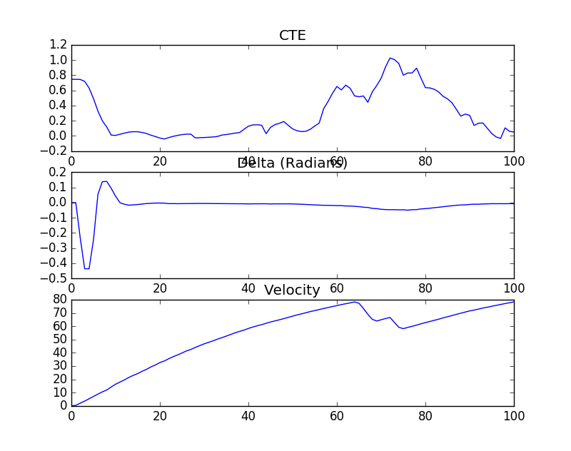
Figure 2 shows the CTE error, Delta (steering angle) and Speed plot for the first 100 iterations on the simulator using the cost function presented above.
In order to deal with the latency, we have to predict the next state before calling the MPC solver. It can be acoomplished using the Model equations. Below, the pseudocode to predict the next state.
dt = 0.1;
x1    = v * cos(0) * dt;
y1    = v * sin(0) * dt;
psi1  = - v/Lf * steer_value * dt;
v1    = throttle_value * dt;
cte1  =   v * sin(epsi1) * dt;
epsi1 = - v * steer_value / Lf * dt;
This video presents the car driving around the track.

