This notebook illustrates the nature of the Stochastic Gradient Descent (SGD) and walks through all the necessary steps to create SGD from scratch in Python. Gradient Descent is an essential part of many machine learning algorithms, including neural networks. To understand how it works you will need some basic math and logical thinking. Though a stronger math background would be preferable to understand derivatives, I will try to explain them as simple as possible.
We will work with the California housing dataset and perform a linear regression to predict apartment prices based on the median income in the block. We will start from the simple linear regression and gradually finish with Stochastic Gradient Descent. So let's get started.
import numpy as np
import pandas as pd
import matplotlib.pyplot as plt
from sklearn.datasets import california_housing
from sklearn.metrics import mean_squared_errorScikit-learn comes with wide variety of datasets for regression, classification and other problems. Lets load our data into pandas dataframe and take a look.
housing_data = california_housing.fetch_california_housing()Features = pd.DataFrame(housing_data.data, columns=housing_data.feature_names)
Target = pd.DataFrame(housing_data.target, columns=['Target'])df = Features.join(Target)Features as MedInc and Target were scaled to some degree.
df.corr().dataframe tbody tr th {
vertical-align: top;
}
.dataframe thead th {
text-align: right;
}
| MedInc | HouseAge | AveRooms | AveBedrms | Population | AveOccup | Latitude | Longitude | Target | |
|---|---|---|---|---|---|---|---|---|---|
| MedInc | 1.000000 | -0.119034 | 0.326895 | -0.062040 | 0.004834 | 0.018766 | -0.079809 | -0.015176 | 0.688075 |
| HouseAge | -0.119034 | 1.000000 | -0.153277 | -0.077747 | -0.296244 | 0.013191 | 0.011173 | -0.108197 | 0.105623 |
| AveRooms | 0.326895 | -0.153277 | 1.000000 | 0.847621 | -0.072213 | -0.004852 | 0.106389 | -0.027540 | 0.151948 |
| AveBedrms | -0.062040 | -0.077747 | 0.847621 | 1.000000 | -0.066197 | -0.006181 | 0.069721 | 0.013344 | -0.046701 |
| Population | 0.004834 | -0.296244 | -0.072213 | -0.066197 | 1.000000 | 0.069863 | -0.108785 | 0.099773 | -0.024650 |
| AveOccup | 0.018766 | 0.013191 | -0.004852 | -0.006181 | 0.069863 | 1.000000 | 0.002366 | 0.002476 | -0.023737 |
| Latitude | -0.079809 | 0.011173 | 0.106389 | 0.069721 | -0.108785 | 0.002366 | 1.000000 | -0.924664 | -0.144160 |
| Longitude | -0.015176 | -0.108197 | -0.027540 | 0.013344 | 0.099773 | 0.002476 | -0.924664 | 1.000000 | -0.045967 |
| Target | 0.688075 | 0.105623 | 0.151948 | -0.046701 | -0.024650 | -0.023737 | -0.144160 | -0.045967 | 1.000000 |
df[['MedInc', 'Target']].describe()[1:] #.style.highlight_max(axis=0).dataframe tbody tr th {
vertical-align: top;
}
.dataframe thead th {
text-align: right;
}
| MedInc | Target | |
|---|---|---|
| mean | 3.482030 | 1.722805 |
| std | 1.364922 | 0.749957 |
| min | 0.499900 | 0.149990 |
| 25% | 2.452025 | 1.119000 |
| 50% | 3.303600 | 1.635000 |
| 75% | 4.346050 | 2.256000 |
| max | 7.988700 | 3.499000 |
It seems that Target has some outliers (as well as MedInc), because 75% of the data has price less than 2.65, but maximum price go as high as 5. We're going to remove extremely expensive houses as they will add unnecessary noize to the data.
df = df[df.Target < 3.5]
df = df[df.MedInc < 8]df[['MedInc', 'Target']].describe()[1:].dataframe tbody tr th {
vertical-align: top;
}
.dataframe thead th {
text-align: right;
}
| MedInc | Target | |
|---|---|---|
| mean | 3.482030 | 1.722805 |
| std | 1.364922 | 0.749957 |
| min | 0.499900 | 0.149990 |
| 25% | 2.452025 | 1.119000 |
| 50% | 3.303600 | 1.635000 |
| 75% | 4.346050 | 2.256000 |
| max | 7.988700 | 3.499000 |
We will also scale MedInc and Target variables to [0-1].
def scale(x):
    min = x.min()
    max = x.max()
    return pd.Series([(i - min)/(max - min) for i in x])

X = scale(df.MedInc)
y = scale(df.Target)X.max(), y.max() # features are scaled now(1.0, 1.0)
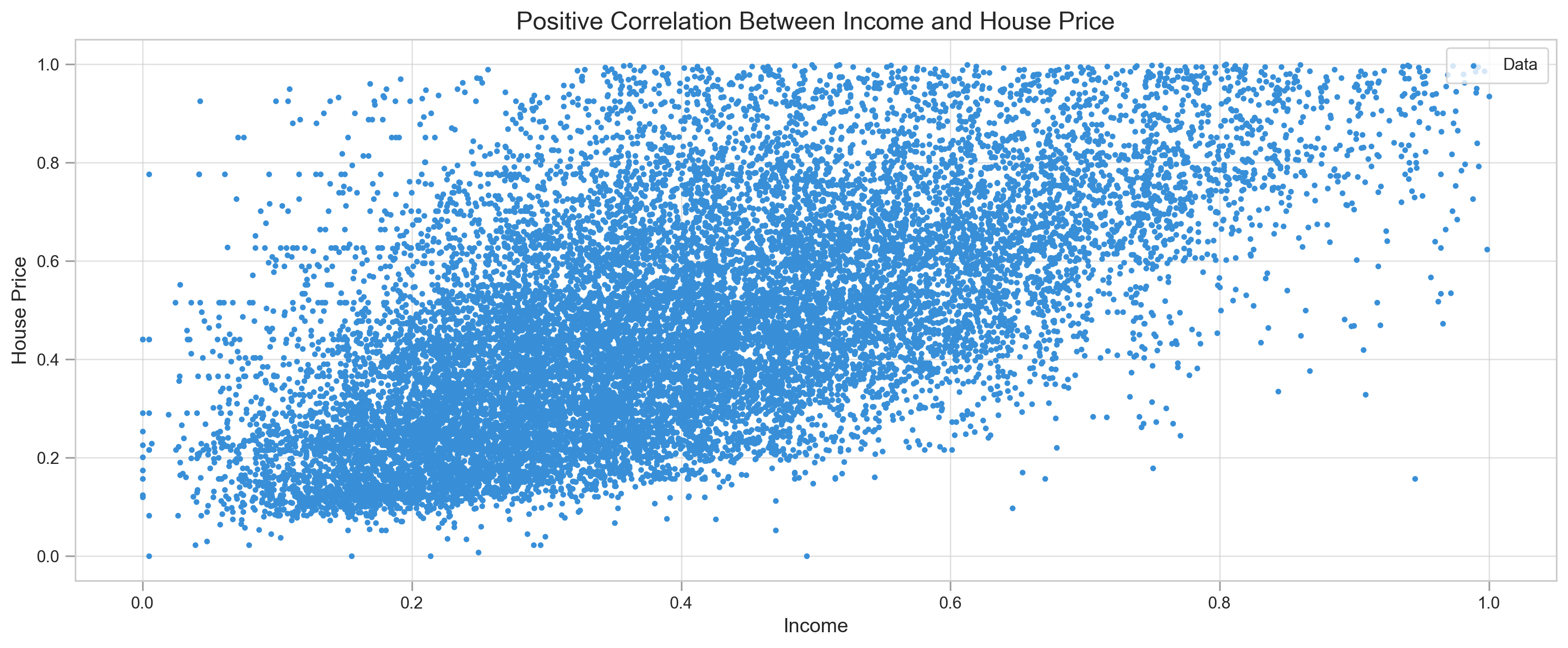
Visually we can determine what kind of accuracy we can expect from the models.
plt.figure(figsize=(16,6))
plt.rcParams['figure.dpi'] = 227
plt.style.use('seaborn-whitegrid')
plt.scatter(X, y, label='Data', c='#388fd8', s=6)
plt.title('Positive Correlation Between Income and House Price', fontSize=15)
plt.xlabel('Income', fontSize=12)
plt.ylabel('House Price', fontSize=12)
plt.legend(frameon=True, loc=1, fontsize=10, borderpad=.6)
plt.tick_params(direction='out', length=6, color='#a0a0a0', width=1, grid_alpha=.6)
plt.show()
Data is quite sparse, but we can still observe some linearity.
Simple linear regression can be described by only two parameters: slope m and intercept b, where x is our median income. Lets take a look at the formulas below:
$$m = \frac{\overline{x}\overline{y}-\overline{xy}}{(\overline{x})^2 - \overline{x^2}} \quad \textrm{and} \quad b = y-mx$$
If we want to add some other features, like size of the apartment, our formula would look like this:
class SimpleLinearRegression:

    def fit(self, X, y):
        self.X = X
        self.y = y
        self.m = ((np.mean(X) * np.mean(y) - np.mean(X*y)) / ((np.mean(X)**2) - np.mean(X**2)))
        self.b = np.mean(y) - self.m * np.mean(X)

    def coeffs(self):
        return self.m, self.b

    def predict(self):
        self.y_pred = self.m * self.X + self.b
        return self.y_pred

    def r_squared(self):
        self.y_mean = np.full((len(self.y)), mean(self.y))
        err_reg = sum((self.y - self.y_pred)**2)
        err_y_mean = sum((self.y - self.y_mean)**2)
        return (1 - (err_reg/err_y_mean))
def plot_regression(X, y, y_pred, log=None, title="Linear Regression"):
plt.figure(figsize=(16,6))
plt.rcParams['figure.dpi'] = 227
plt.scatter(X, y, label='Data', c='#388fd8', s=6)
if log != None:
for i in range(len(log)):
plt.plot(X, log[i][0]*X + log[i][1], lw=1, c='#caa727', alpha=0.35)
plt.plot(X, y_pred, c='#ff7702', lw=3, label='Regression')
plt.title(title, fontSize=14)
plt.xlabel('Income', fontSize=11)
plt.ylabel('Price', fontSize=11)
plt.legend(frameon=True, loc=1, fontsize=10, borderpad=.6)
plt.tick_params(direction='out', length=6, color='#a0a0a0', width=1, grid_alpha=.6)
plt.show()X = df.MedInc
y = df.Targetlr = SimpleLinearRegression()lr.fit(X, y)y_pred = lr.predict()print("MSE:",mean_squared_error(y, y_pred))
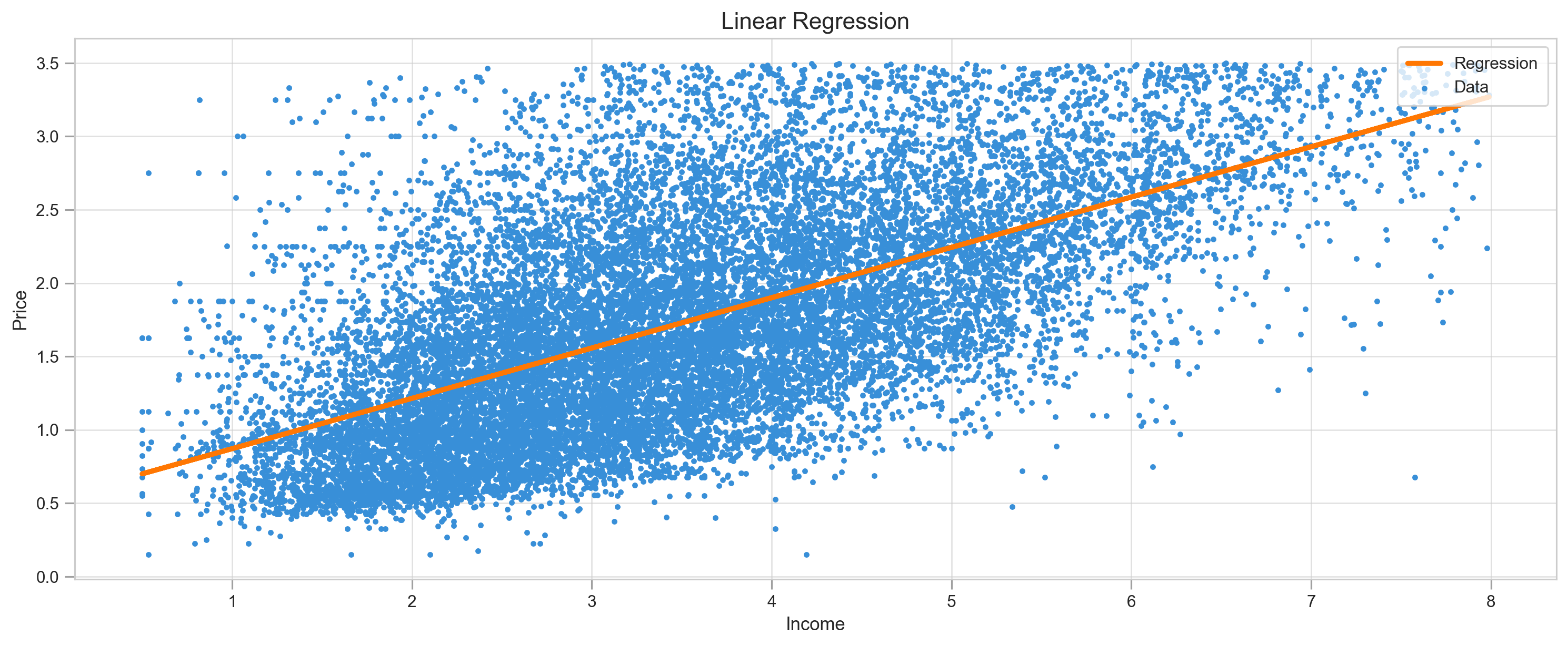
plot_regression(X, y, y_pred, title="Linear Regression")MSE: 0.34320521502255963
Result of our model is the regression line. Just by looking at the graph we can tell that data points go well above and beyond our line, making predictions approximate.
Similar to from sklearn.linear_model import LinearRegression, we can calculate coefficients with Least Squares method. Numpy can calculate this formula almost instantly (of course depends on the amount of data) and precise.
X = df.drop('Target', axis=1) # matrix A, or all the features
y = df.Targetclass MultipleLinearRegression:
'''
Multiple Linear Regression with Least Squares
'''
def fit(self, X, y):
X = np.array(X)
y = np.array(y)
self.coeffs = np.linalg.inv(X.T.dot(X)).dot(X.T).dot(y)
def predict(self, X):
X = np.array(X)
result = np.zeros(len(X))
for i in range(X.shape[1]):
result += X[:, i] * self.coeffs[i]
return result
def coeffs(self):
return self.coeffsmlp = MultipleLinearRegression()mlp.fit(X, y)y_pred = mlp.predict(X)mean_squared_error(y, y_pred)0.2912984534321039
The idea behind gradient descent is simple - by gradually tuning parameters, such as slope (m) and the intercept (b) in our regression function y = mx + b, we minimize cost.
By cost, we usually mean some kind of a function that tells us how far off our model predicted result. For regression problems we often use mean squared error (MSE) cost function. If we use gradient descent for the classification problem, we will have a different set of parameters to tune.
$$ MSE = \frac{1}{n}\sum_{i=1}^{n} (y_i - \hat{y_i})^2 \quad \textrm{where} \quad \hat{y_i} = mx_i + b $$
Now we have to figure out how to tweak parameters m and b to reduce MSE.
We use partial derivatives to find how each individual parameter affects MSE, so that's where word partial comes from. In simple words, we take the derivative with respect to m and b separately. Take a look at the formula below. It looks almost exactly the same as MSE, but this time we added f(m, b) to it. It essentially changes nothing, except now we can plug m and b numbers into it and calculate the result.
This formula (or better say function) is better representation for further calculations of partial derivatives. We can ignore sum for now and what comes before that and focus only on
With respect to m means we derive parameter m and basically ignore what is going on with b, or we can say its 0. To derive with respect to m we will use chain rule.
Chain rule applies when one function sits inside of another. If you're new to this, you'd be surprised that
- Derivative of
$()^2$ is$2()$ , same as$x^2$ becomes$2x$ - We do nothing with
$y - (mx + b)$ , so it stays the same - Derivative of
$y - (mx + b)$ with respect to m is$(0 - (x + 0))$ or$-x$ , because y and b are constants, they become 0, and derivative of mx is x
Multiply all parts we get following:
Here,
Same rules apply to the derivative with respect to b.
-
$()^2$ becomes$2()$ , same as$x^2$ becomes$2x$ -
$y - (mx + b)$ stays the same -
$y - (mx + b)$ becomes$(0 - (0 + 1))$ or$-1$ , because y and mx are constants, they become 0, and derivative of b is 1
Multiply all the parts together and we get
Few details we should discuss befor jumping into code:
- Gradient descent is an iterative process and with each iteration (
epoch) we slightly minimizing MSE, so each time we use our derived functions to update parametersmandb - Because its iterative, we should choose how many iterations we take, or make algorithm stop when we approach minima of MSE. In other words when algorithm is no longer improving MSE, we know it reached minimum.
- Gradient descent has an additional parameter learning rate (
lr), which helps control how fast or slow algorithm going towards minima of MSE
Thats about it. So you can already understand that Gradient Descent for the most part is just process of taking derivatives and using them over and over to minimize function.
def gradient_descent(X, y, lr=0.05, epoch=10):
'''
Gradient Descent for a single feature
'''
m, b = 0.2, 0.2 # parameters
log, mse = [], [] # lists to store learning process
N = len(X) # number of samples
for _ in range(epoch):
f = y - (m*X + b)
# Updating m and b
m -= lr * (-2 * X.dot(f).sum() / N)
b -= lr * (-2 * f.sum() / N)
log.append((m, b))
mse.append(mean_squared_error(y, (m*X + b)))
return m, b, log, mseX = df.MedInc
y = df.Target
m, b, log, mse = gradient_descent(X, y, lr=0.01, epoch=100)
y_pred = m*X + b
print("MSE:",mean_squared_error(y, y_pred))
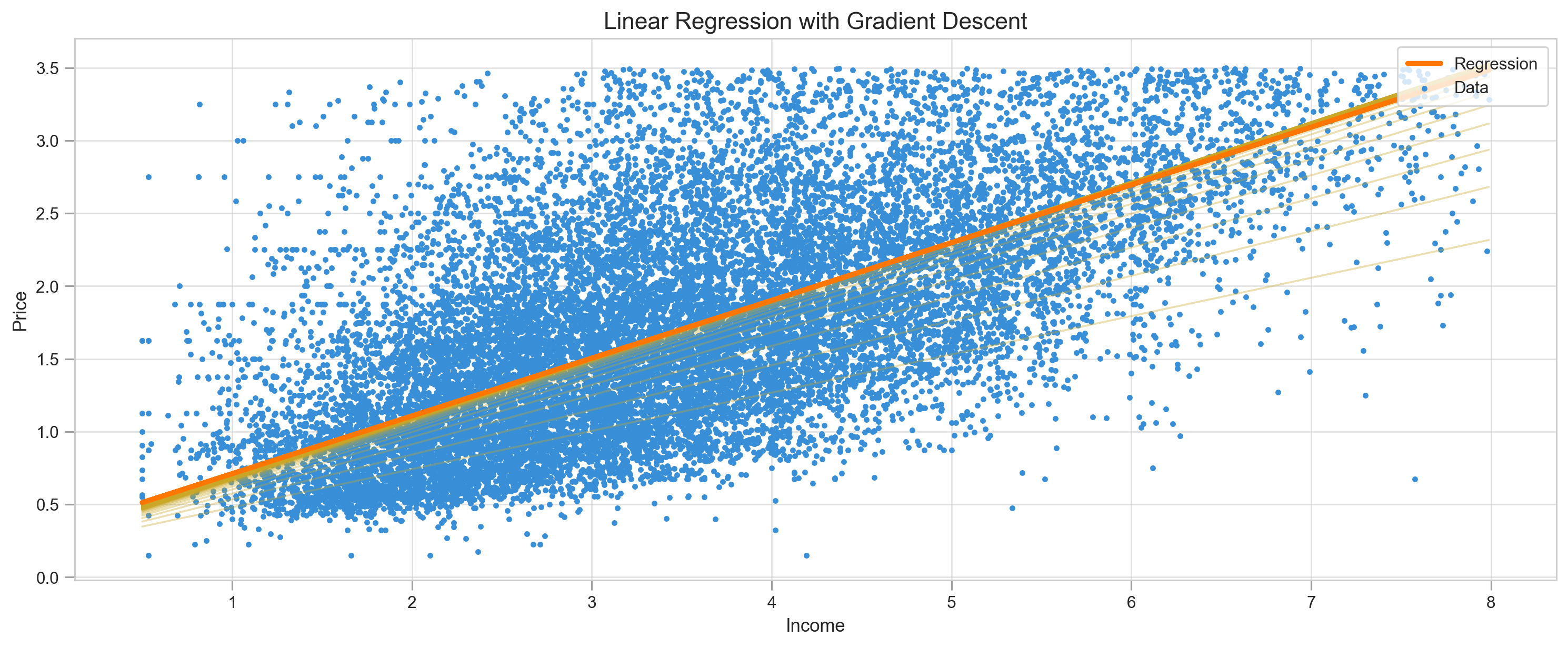
plot_regression(X, y, y_pred, log=log, title="Linear Regression with Gradient Descent")
plt.figure(figsize=(16,3))
plt.rcParams['figure.dpi'] = 227
plt.plot(range(len(mse)), mse)
plt.title('Gradient Descent Optimization', fontSize=14)
plt.xlabel('Epochs')
plt.ylabel('MSE')
plt.show()MSE: 0.3493097403876614
Stochastic Gradient Descent works almost the same as Gradient Descent (also called Batch Gradient Descent), but instead of training on entire dataset, it picks only one sample to update m and b parameters, which makes it much faster. In the function below I made possible to change sample size (batch_size), because sometimes its better to use more than one sample at a time.
def SGD(X, y, lr=0.05, epoch=10, batch_size=1):
'''
Stochastic Gradient Descent for a single feature
'''
m, b = 0.5, 0.5 # initial parameters
log, mse = [], [] # lists to store learning process
for _ in range(epoch):
indexes = np.random.randint(0, len(X), batch_size) # random sample
Xs = np.take(X, indexes)
ys = np.take(y, indexes)
N = len(Xs)
f = ys - (m*Xs + b)
# Updating parameters m and b
m -= lr * (-2 * Xs.dot(f).sum() / N)
b -= lr * (-2 * f.sum() / N)
log.append((m, b))
mse.append(mean_squared_error(y, m*X+b))
return m, b, log, msem, b, log, mse = SGD(X, y, lr=0.01, epoch=100, batch_size=2)y_pred = m*X + b
print("MSE:",mean_squared_error(y, y_pred))
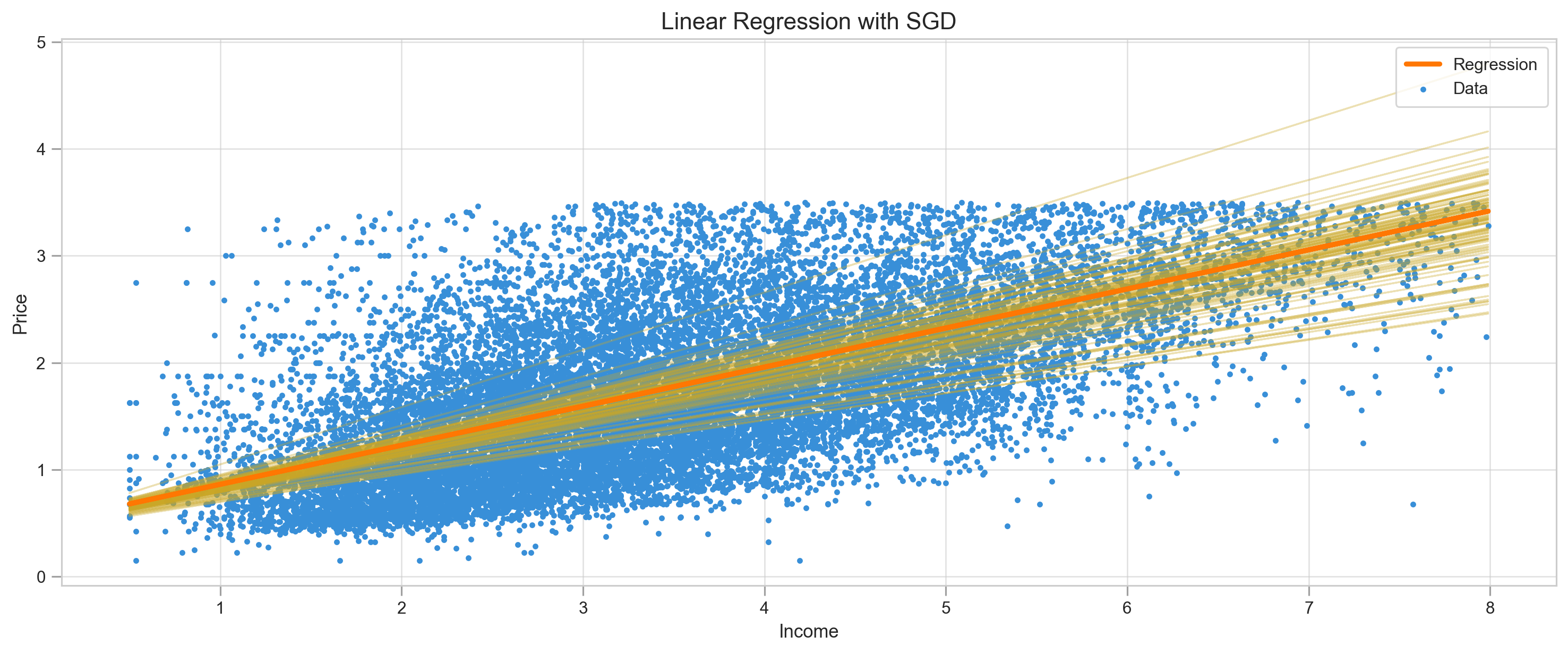
plot_regression(X, y, y_pred, log=log, title="Linear Regression with SGD")
plt.figure(figsize=(16,3))
plt.rcParams['figure.dpi'] = 227
plt.plot(range(len(mse)), mse)
plt.title('SGD Optimization', fontSize=14)
plt.xlabel('Epochs', fontSize=11)
plt.ylabel('MSE', fontSize=11)
plt.show()MSE: 0.3462919845446769
We can observe how regression line went up and down to find right parameters and MSE not as smooth as regular gradient descent.
X = df.MedInc
y = df.TargetX = np.concatenate((X,X,X,X,X,X,X,X,X,X,X,X,X,X,X,X,X))
y = np.concatenate((y,y,y,y,y,y,y,y,y,y,y,y,y,y,y,y,y))X.shape, y.shape((304946,), (304946,))
%timeit SGD(X, y, lr=0.01, epoch=1000, batch_size=1)1.22 s ± 8.95 ms per loop (mean ± std. dev. of 7 runs, 1 loop each)
%timeit gradient_descent(X, y, lr=0.01, epoch=1000)2.02 s ± 79.4 ms per loop (mean ± std. dev. of 7 runs, 1 loop each)
- SGD is twice as fast as Gradient Descent (also called Batch Gradient Descent)
- On sparse data, we can increase the batch size to speed up learning process. It's not a pure form of SGD, but we can call it a mini-batch SGD
- Smaller learning rate helps to prevent overfitting but can be adjusted accordingly


