complex-plotting-tools

Module for plotting complex-valued functions of complex variable using different methods.

Examples gallery

A script for generating the following examples can be found at examples.py.

To use this module just place the script cplotting_tools.py in your working directory. It can be imported like this:

import cplotting_tools as cplt

In this first set of examples the test function is the following one:

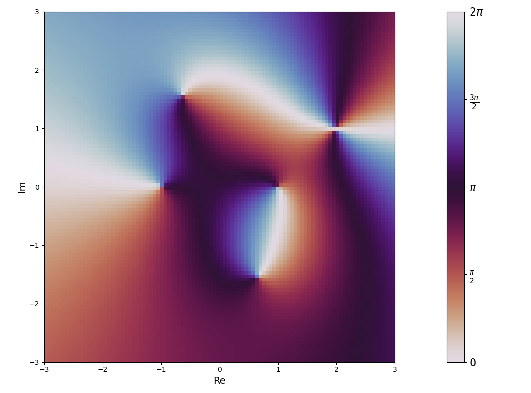
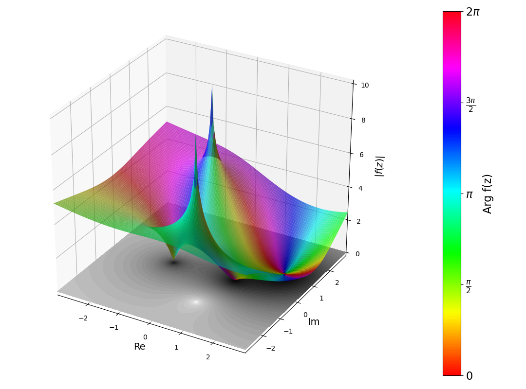
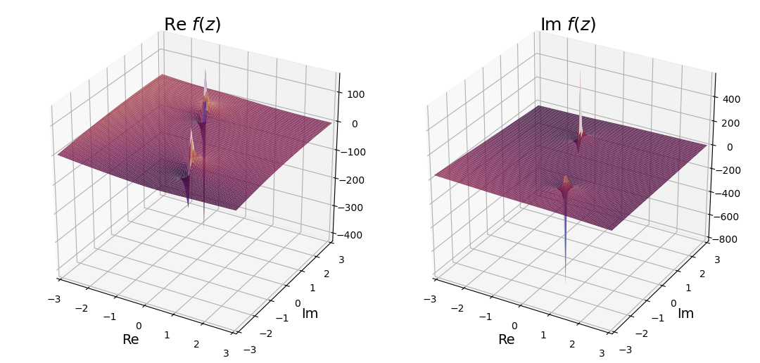
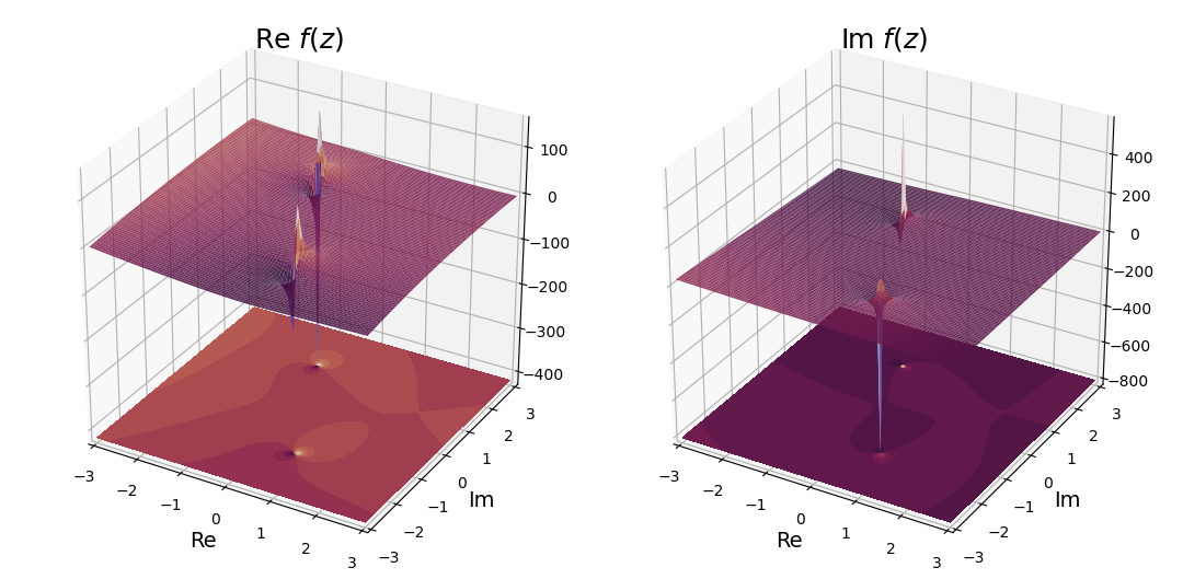
$$ f(z) = \dfrac{(z^2-1)(z-2-i)^2}{z^2+2+2i} $$

We start defining the variables and parameters for these first examples:

import numpy as np

N = 100
lim = 3
x, y = np.meshgrid(np.linspace(-lim,lim,N), 
                   np.linspace(-lim,lim,N))
z = x + 1j*y

The code of the function $f$ , f, and its set of poles and zeros, pts, looks like this:

f = (z**2-1)*(z-2-1j)**2/(z**2+2+2j)
pts = [-1, 1, 2+1j, 2**(3/4)*np.exp(1j*(5*np.pi/8)), 2**(3/4)*np.exp(1j*(5*np.pi/8+np.pi))]

Then, we can use the functions defined in cplotting_tools.py to generate, for example, the following plots:

`cplt.domain_coloring(x, y, f, cmap="hsv")`	`cplt.domain_coloring(x, y, f, cmap="twilight_r")`
`cplt.domain_coloring_illuminated(x, y, f, log_brightness=False)`	`cplt.domain_coloring_illuminated(x, y, f)`
`cplt.complex_plot3D(x, y, f, log_mode=False)`	`cplt.complex_plot3D(x, y, f, log_mode=True)`
`cplt.plot_re_im(x, y, f, cmap="twilight", contour=False, alpha=0.9)`	`cplt.plot_re_im(x, y, f, cmap="twilight", contour=True, alpha=0.9)`
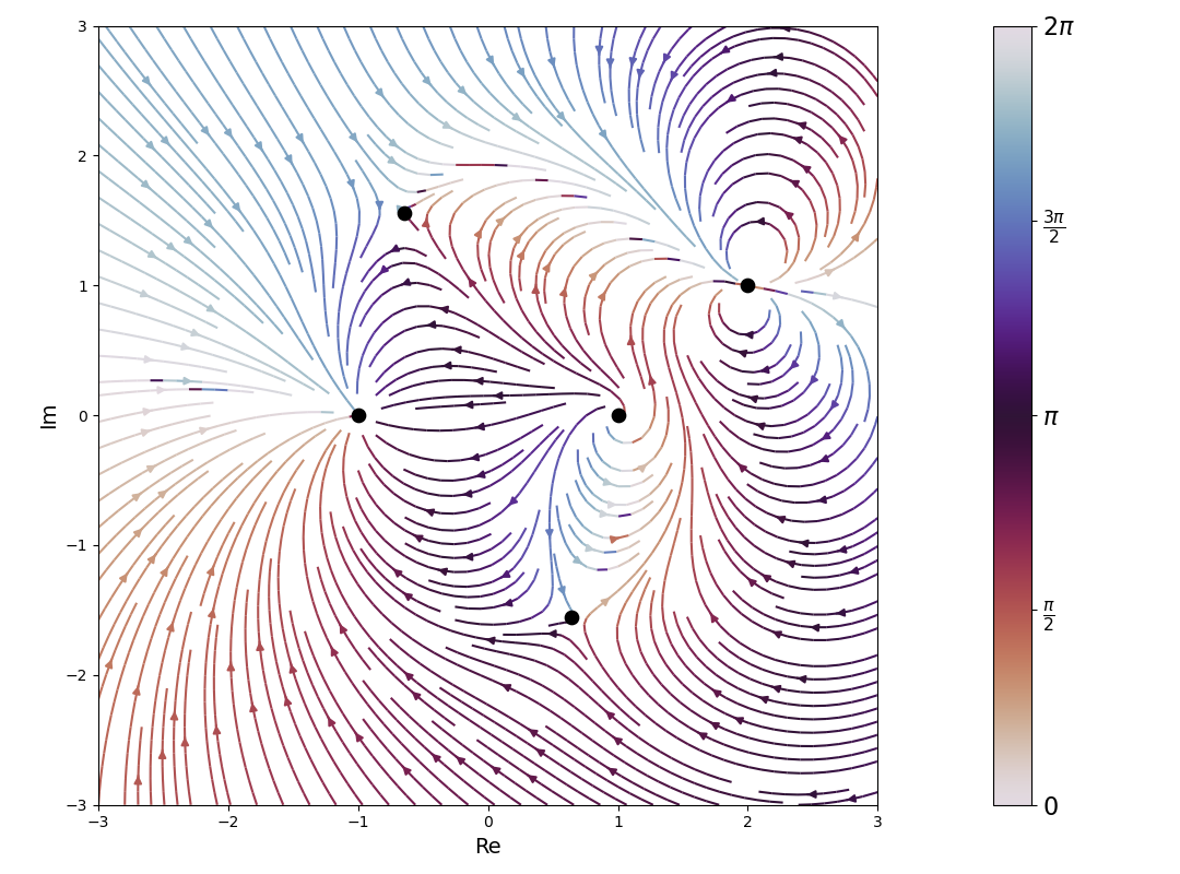
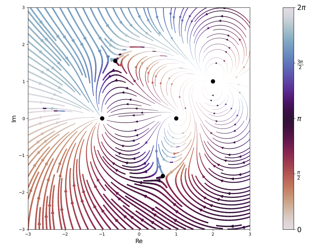
`cplt.complex_streamplot(x, y, f, mod_as_linewidths=False, cmap="twilight_r", density=2, scatterpoints=pts)`	`cplt.complex_streamplot(x, y, f, mod_as_linewidths=True, cmap="twilight_r", density=2, scatterpoints=pts)`
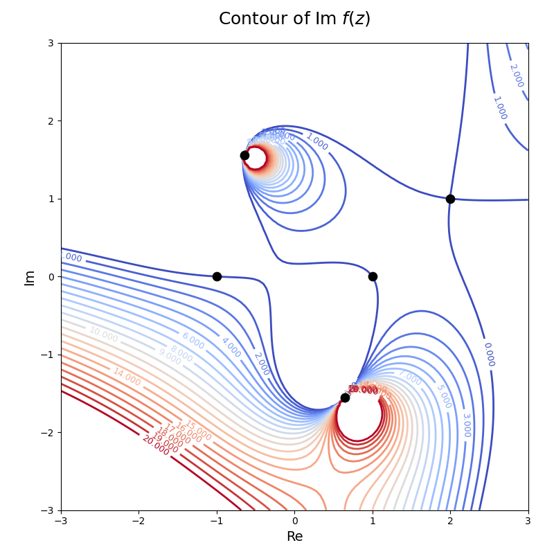
`cplt.complex_contour(x, y, f, mode="real", levels=np.arange(0,21,1), lw=2, cmap="coolwarm", scatterpoints=pts)`	`cplt.complex_contour(x, y, f, mode="imag", levels=np.arange(0,21,1), lw=2, cmap="coolwarm", scatterpoints=pts)`
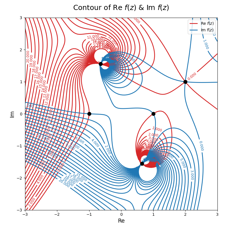
`cplt.complex_contour(x, y, f, mode="modulus", levels=np.arange(0,21,1), lw=2, cmap="coolwarm", scatterpoints=pts)`	`cplt.complex_contour(x, y, f, mode="both", levels=np.arange(0,21,1), lw=2, cmap="coolwarm", scatterpoints=pts)`

In this second set of examples the test function is:

$$ f(z)=\cos z $$

As we did in the first set of examples, we start defining the variables, the parameters and the function:

N = 40
lim = 6
x, y = np.meshgrid(np.linspace(-lim,lim,N), 
                    np.linspace(-lim,lim,N))
z = x + 1j*y
f = np.cos(z)

Then, we could obtain the following plots:

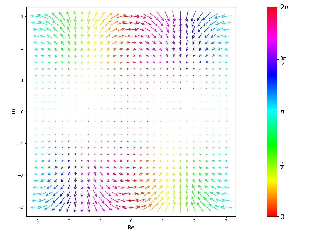
`cplt.complex_vector_field(x, y, f, norm=False)`	`cplt.complex_vector_field(x, y, f, cmap="hsv", norm=False)`
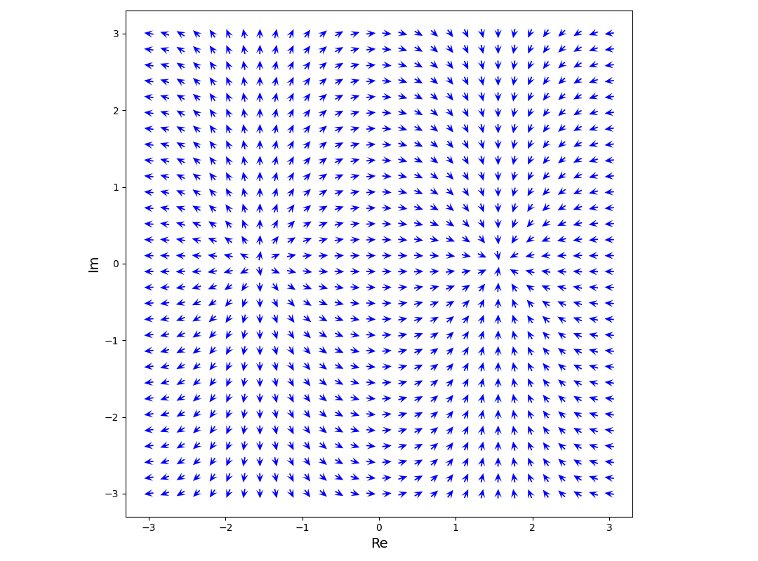
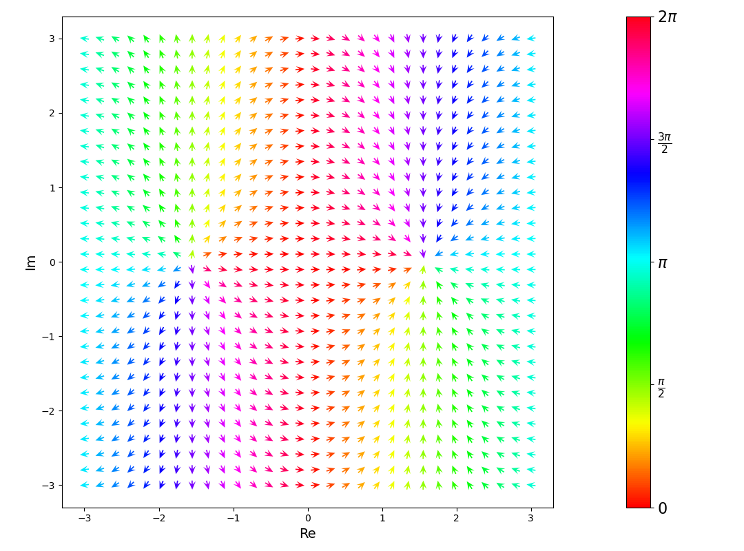
`cplt.complex_vector_field(x, y, f, norm=True)`	`cplt.complex_vector_field(x, y, f, cmap="hsv", norm=True)`

If you are a beginner with complex functions you might also find useful: "Plotting Complex Variable Functions".

I would also like to recommend an online interactive book by Juan Carlos Ponce Campuzano called "COMPLEX ANALYSIS - A Visual and Interactive Introduction".