The goals / steps of this project are the following:
- Compute the camera calibration matrix and distortion coefficients given a set of chessboard images.
- Apply a distortion correction to raw images.
- Use color transforms, gradients, etc., to create a thresholded binary image.
- Apply a perspective transform to rectify binary image ("birds-eye view").
- Detect lane pixels and fit to find the lane boundary.
- Determine the curvature of the lane and vehicle position with respect to center.
- Warp the detected lane boundaries back onto the original image.
- Output visual display of the lane boundaries and numerical estimation of lane curvature and vehicle position.
The images for camera calibration are stored in the folder called camera_cal. The images in test_images are for testing your pipeline on single frames.
The main objective is to run the above steps as a pipleline and run this on the project video .
The code for this pipline is written in an ipython note book called AdvanceLaneline.ipynb
###Camera Calibration
As first step we calibrate the camera to avoid any distortion.
The code for this step is contained in the first code cell of the IPython notebook located in "./examples/example.ipynb" (or in lines # through # of the file called some_file.py).
I start by preparing "object points", which will be the (x, y, z) coordinates of the chessboard corners in the world. Here I am assuming the chessboard is fixed on the (x, y) plane at z=0, such that the object points are the same for each calibration image. Thus, objp is just a replicated array of coordinates, and objpoints will be appended with a copy of it every time I successfully detect all chessboard corners in a test image. imgpoints will be appended with the (x, y) pixel position of each of the corners in the image plane with each successful chessboard detection.
I then used the output objpoints and imgpoints to compute the camera calibration and distortion coefficients using the cv2.calibrateCamera() function. I applied this distortion correction to the test image using the cv2.undistort() function and obtained this result:
ret, mtx, dist, rvecs, tvecs = cv2.calibrateCamera(objpoints, imgpoints, img_size,None,None)
dst = cv2.undistort(img, mtx, dist, None, mtx)
As you can see I have calibrated the chess board based on the number of x and y's in the chess board.
Based on the expected X's and Y's callibration is applied and you can see here that theimage to the right is claibrated.
###Pipeline
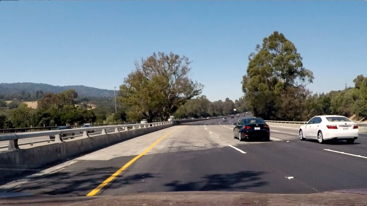
For an example we are going to use the following image to show every step in the pipeline.

As the first step the image that come in to the pipline are calibrated to avoid any kind of distortion. We then later apply computer vision based image filter.
As a first step I find the the sobel'y' and soble'y' and get the image filter with respect to the S(saturation) and v(value) which are not in the RBG color space rather in the HLS and HSV color space . Example we have the image transformation in and get the binary transformation.
 Later I perform a color transformation and get the binary output.
I filter all these output based on trials and look for image with the best lane marking .
    preprocessImage = np.zeros_like(image[:,:,0])
    gradx = abs_sobel_thresh(image, orient='x', sobel_kernel=ksize, thresh=(5, 255))
    grady = abs_sobel_thresh(image, orient='y', sobel_kernel=ksize, thresh=(7, 255))
    c_binary = color_threshold(image,sthresh=(150,255),vthresh=(220,255))
    #conbining all the filters
    preprocessImage[((gradx ==1)&(grady ==1)|(c_binary==1))] = 255
gradx grady and c_binary are filters that are later merged to the preprocessImage image which can be in the last of the code above.
Once the transformation is done we look into the region of intrest . Here I assume the region based of a certain percentage with respect to the original image.
image_size = (image.shape[1],image.shape[0])
    bottomWidth = .76   # percent of bottom trapizoied height
    midWidth= .08       #percent of middle trapizoid height
    hightPicture = .62  # percent of trapizoid height
    bottomTrim = 0.935  # percent from top to bottom to avoid car hood
    src = np.float32([[image.shape[1] * (.5 - midWidth / 2),image.shape[0] * hightPicture],
                      [image.shape[1] * (.5 + midWidth / 2),image.shape[0] * hightPicture],
                      [image.shape[1] * (.5 + bottomWidth / 2),image.shape[0] * bottomTrim],
                      [image.shape[1] * (.5 - bottomWidth / 2),image.shape[0] * bottomTrim]])
    offset =image_size[0] *.15
    dst = np.float32([[offset,0],[image_size[0]-offset,0],[image_size[0]-offset,image_size[1]],[offset,image_size[1]]])
The bottomWidth,midWidth, hightPicture,bottomTrim are used to compute the boundry for the trapazoid. src is the coordiantes of the trapazoid .
Using Perpective image transformation we would line to transform that bounded trapezoid to a rectangular image that be used see as a bird eye/ . For that to happen we need to mention the destination shape which is dst in my code.
Once src and dst is computed we can make the pespective transform which is this
    M = cv2.getPerspectiveTransform(src,dst)
    Minv = cv2.getPerspectiveTransform(dst,src)
    warped = cv2.warpPerspective(preprocessImage,M,image_size ,flags=cv2.INTER_LINEAR)
M is used to convert the perspective image to the required shape and its inverse is also computed for us in later to perform a reverse transformation.
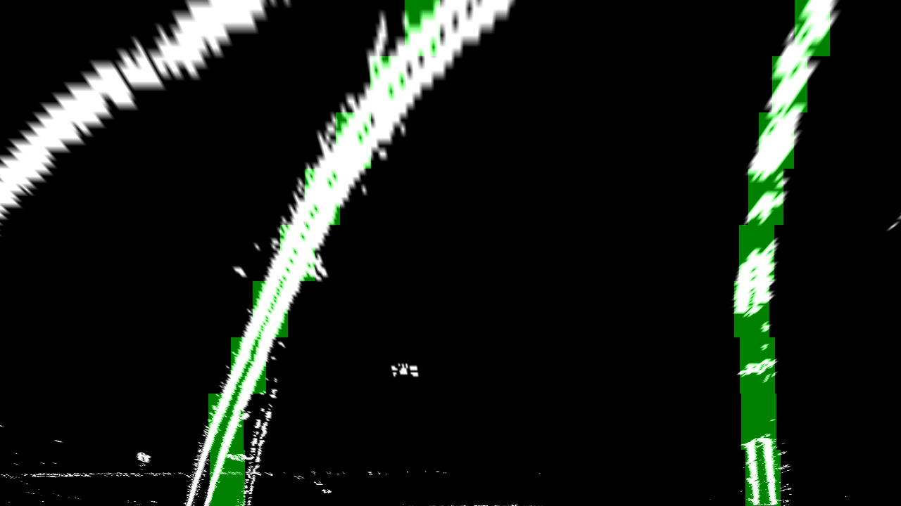
Once I have the new transformed image I should be able to see the image two parallel lines which i detect using a sliding window and compute the centroid od the window with respect to all other point that are availble in that window.
For each of these images that is transformed the list of centroids are calculated and are saved in a class object called tracker. I map these point onto the transformed image.

The centroid are polyfitted and to get an equation of a line and use the equation to map perspective image.
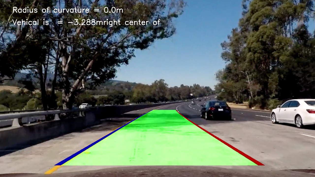
Once pollyfitted the point are mapped back or apply inverse perspective after detection and map that to the original image.
road_wrapped = cv2.warpPerspective(road,Minv,image_size,flags=cv2.INTER_LINEAR)After this using these point i display the region covered by lanes.

You can check out the video that undergoes this pipeline to detect the lane lines. Here's a link to my video result
###Considerations , Issues ,Problem and Future Enhancement
The sample vidoe is a very good example to find the lanes. Though this experment would have had a bad result in case the there was high traffic such as i urban area. I one case my pipeline did perforem well where there was sudden shadow and the lane line are barely visible.
I feel that in such cases a few extra points can be interpolated so that the lane prediction is not off only in such exteme cases.
As an enhancement I would like to implement senario based image brightness correction . Also I feel that that the bounding box for searching the lanes can be made shorter so as to detect accurate lane markings.


