MDMr: Multiregression Dynamic Models in R

MDM is a Bayesian dynamic regression model used to estimate effective connectivity between variables over time. Currently, this software employs the reticulate package to establish a connection between the GOBNILP algorithm and the R software.

Any suggestions to improve the package are appreciated! If you have any, please send an email to the package maintainer.

Installation

To install the Multiregression Dynamic Models package mdmr from the development version on GitHub, just use the command:

# install.packages("devtools")
devtools::install_github("arzevedo/mdmr")

Once you have the mdmr package installed, you must install Python on your machine if you haven't already. It's recommended that you use the reticulate package:

reticulate::install_python()

Next, you should build an environment with the sole purpose of running the GOBNILP algorithm. You can do this with the following code to install the pygobnilp package in your environment.

The first argument is the name of the environment, and the second is the package:

reticulate::virtualenv_install("r-reticulate", "pygobnilp")

Once you've installed everything you need, you can access Python from the environment using the following function:

reticulate::use_virtualenv("r-reticulate")

If you encounter any problems with the code above, you can go to the reticulate official website and check the documentation.

Data input

The data input must adhere to a specific format for the package to work properly. In the case of a single subject, you may use a dataframe or matrix class as input. In a more complex setting, it's important that the input has three dimensions. The array class will satisfy this condition. The first dimension of the array must represent the timepoints of the timeseries, the second dimension must represent the nodes or variables of each timeseries, and the third dimension represents the subjects.

If your data is not currently in this format, please make the necessary adjustments.

You can access a simple simulation example with 197 observations, 4 nodes, and 2 subjects as follows:

library(mdmr)
simulated_data <- mdmr::dts_4n

dimnames(simulated_data)[[2]] <- paste0("var", 1:4)

sim_mdm_score <- mdm_score(data_input = simulated_data, GOLB_print = TRUE, subjects_length = 2)

A built-in application

First, load the package. mdmr has a built-in dataset that consists of new weekly COVID-19 cases in the five macroregions of Brazil until March 2023.

library(mdmr)
covid_data <- mdmr::regioes

Next, you can calculate the scores for the network:

mdmModel <- mdm_score(covid_data, GOLB_print = TRUE)

This saves a text file in your environment. This file will be used by the GOBNILP algorithm. Now, you can use the run_BN_pygobnilp function to obtain the adjacency matrix:

adj_matrix_GOB <- mdmr::run_BN_pygobnilp("mdm_score_07_ago_2023", palim = 5)
m_ad <- adj_matrix_GOB$wide

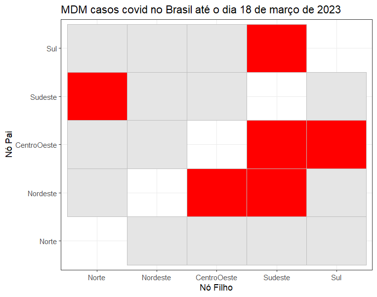
To visualize the static structure, you could use the ggplot package:

library(tidyverse)
adj_matrix_GOB$long |>
      mutate(
            value = if_else(round(Value) == 1, 1, 0)
      ) |>
      mutate(Father = factor(Father, levels = c(
            "Norte", "Nordeste", "CentroOeste", "Sudeste", "Sul"
      )),
      Child = factor(Child, levels = c(
            "Norte", "Nordeste", "CentroOeste", "Sudeste", "Sul"
      ))) |>
      ggplot(aes(y = Father, x = Child, fill = factor(value))) +
      geom_tile(color = "gray") +
      scale_fill_manual(values = c("0" = "gray90", "1" = "red")) +
      theme_bw() +
      labs(y = "Nó Pai", x = "Nó Filho", fill = NULL,
           title = "MDM casos covid no Brasil até o dia 18 de março de 2023")+
      theme(legend.position = "none")

The next step requires a reordering of the data input:

covid_data <- covid_data[,sort(colnames(covid_data))]

Find the discount factor that maximizes the LPL:

DF = mdmr::CDELT(dts = as.matrix(covid_data), m_ad = m_ad)

Now we use the mdm_filt function to collect the dynamic parameters:

Filt = mdmr::mdm_filt(
      # Data input
      dts = as.matrix(covid_data),
      # Adjacency matrix
      # It's important that the adjacency matrix follows the order of the data input
      m_ad = m_ad,
      # Estimated discount factor
      DF$DF_hat)

And finally, it's possible to smooth the distributions:

Smoo = mdmr::mdm_smoo(Filt$mt, Filt$Ct, Filt$Rt, Filt$nt, Filt$dt)

# Bind all parameters togheter
all_betas <- t(Reduce(x = Smoo$smt, rbind))

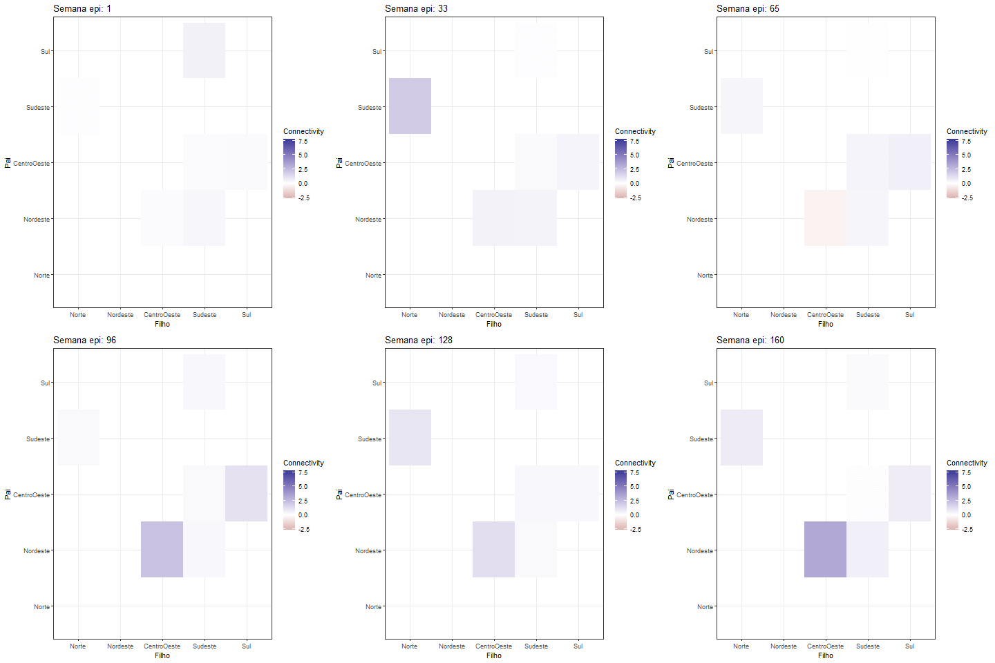
To enhance comprehension of the model's output and effectively interpret the outcomes, it could be beneficial to create visualizations representing select connectivity parameters:

as_tibble(all_betas) |> 
      ggplot(aes(x = 1:160)) +
      #geom_line(aes(y = beta0_Sul), color = "blue") +
      geom_line(aes(y = `Sul->Sudeste`), color = "firebrick") +
      geom_line(aes(y = `CentroOeste->Sul`), color = "navy") +
      labs(x = "Epi Week", y = "beta")+
      theme_bw()

Creating a GIF of the heatmap offers a fascinating approach to visually represent the dynamic interactions among variables in the MDM model:

library(gganimate)

fix_plot <- all_betas |> as_tibble() |> 
      select(contains("->")) |> mutate(id = 1:dim(all_betas)[1]) |>
      pivot_longer(cols = - id) |>
      tidyr::separate(col = name, into = c("Father", "Child"), sep = "->") |>
      mutate(
            Father = factor(Father, levels = c(
                  "Norte", "Nordeste", "CentroOeste", "Sudeste", "Sul"
            )),
            Child = factor(Child, levels = c(
                  "Norte", "Nordeste", "CentroOeste", "Sudeste", "Sul"
            ))
      ) |>
      ggplot(aes(y = Father, x = Child, fill = value)) +
      geom_tile() +
      scale_y_discrete(drop=FALSE) +
      scale_x_discrete(drop=FALSE) +
      scale_fill_gradient2()+
      #scale_fill_viridis_c() +  # You can change the color scale if you prefer
      labs(title = "Semana epi: {frame_time}", x = "Filho", y = "Pai",
           fill = "Connectivity")+
      theme_bw()

animation <- fix_plot +
      transition_time(id) +
      ease_aes('linear'#, interval = 0.5
      )

print(animation)

Acknowledgments

The development of this R package was done in collaboration with Dr. Lilia Costa and Mariana Almeida.

Bibliography

To learn more about the methods and how they work please check.

Costa, L., Smith, J., Nichols, T., Cussens, J., Duff, E.P. and Makin, T.R., 2015. Searching multiregression dynamic models of resting-state fMRI networks using integer programming.

Cussens, J. and Bartlett, M., 2015. GOBNILP 1.6. 2 User/Developer Manual1. University of York.

Cussens, J., 2020, February. GOBNILP: Learning Bayesian network structure with integer programming. In International Conference on Probabilistic Graphical Models (pp. 605-608). PMLR.

Cussens, J., pygobnilp manual (version 1.0).

West, M. and Harrison, J., 2006. Bayesian forecasting and dynamic models. Springer Science & Business Media.