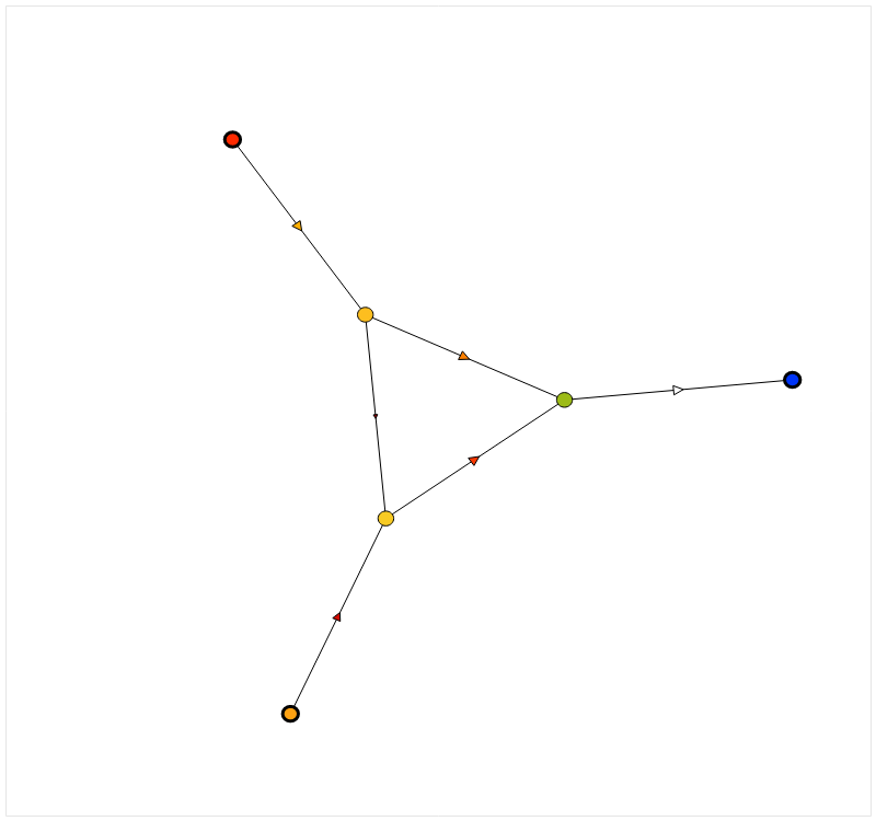
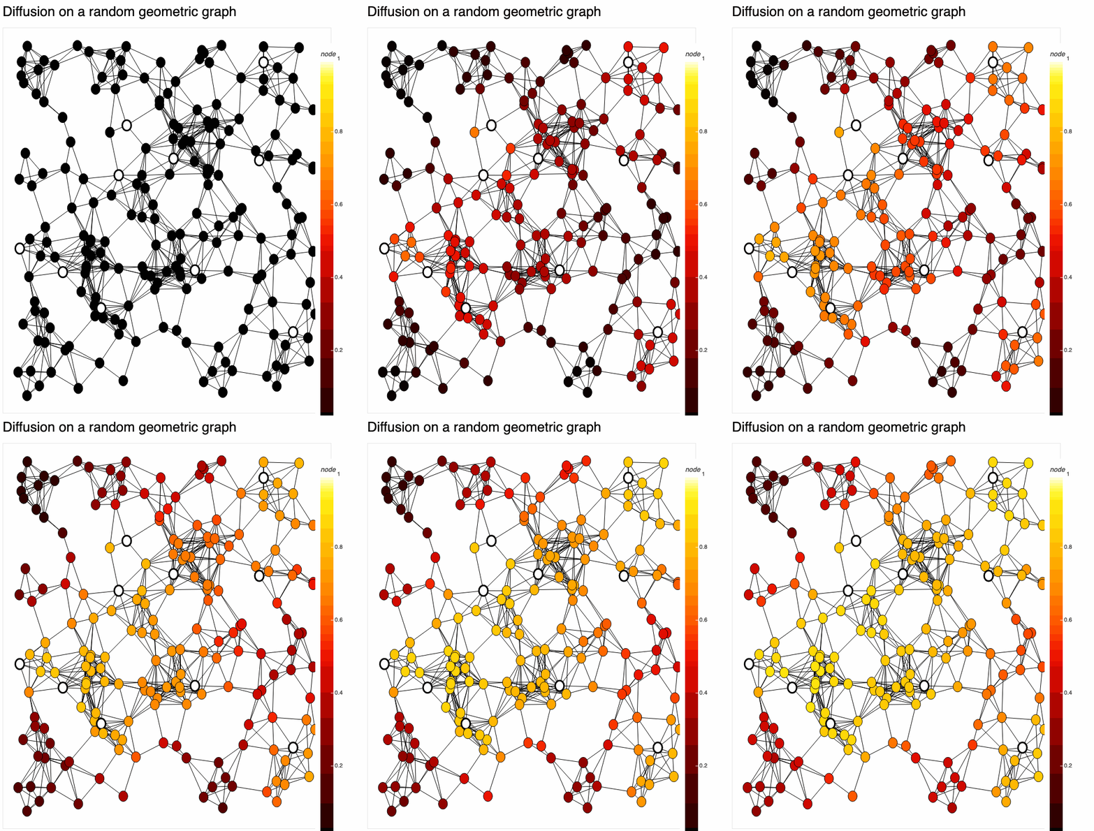
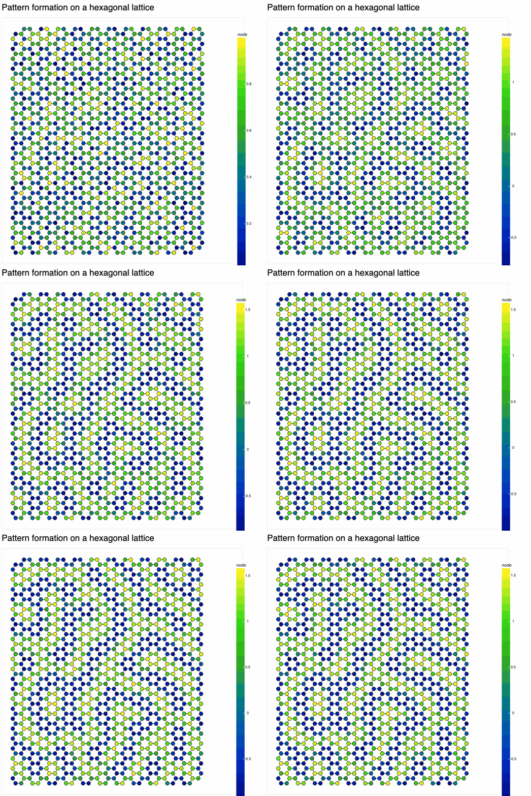
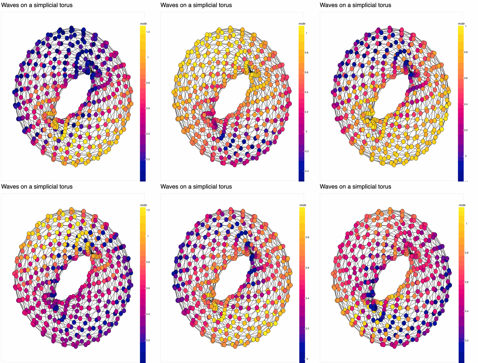
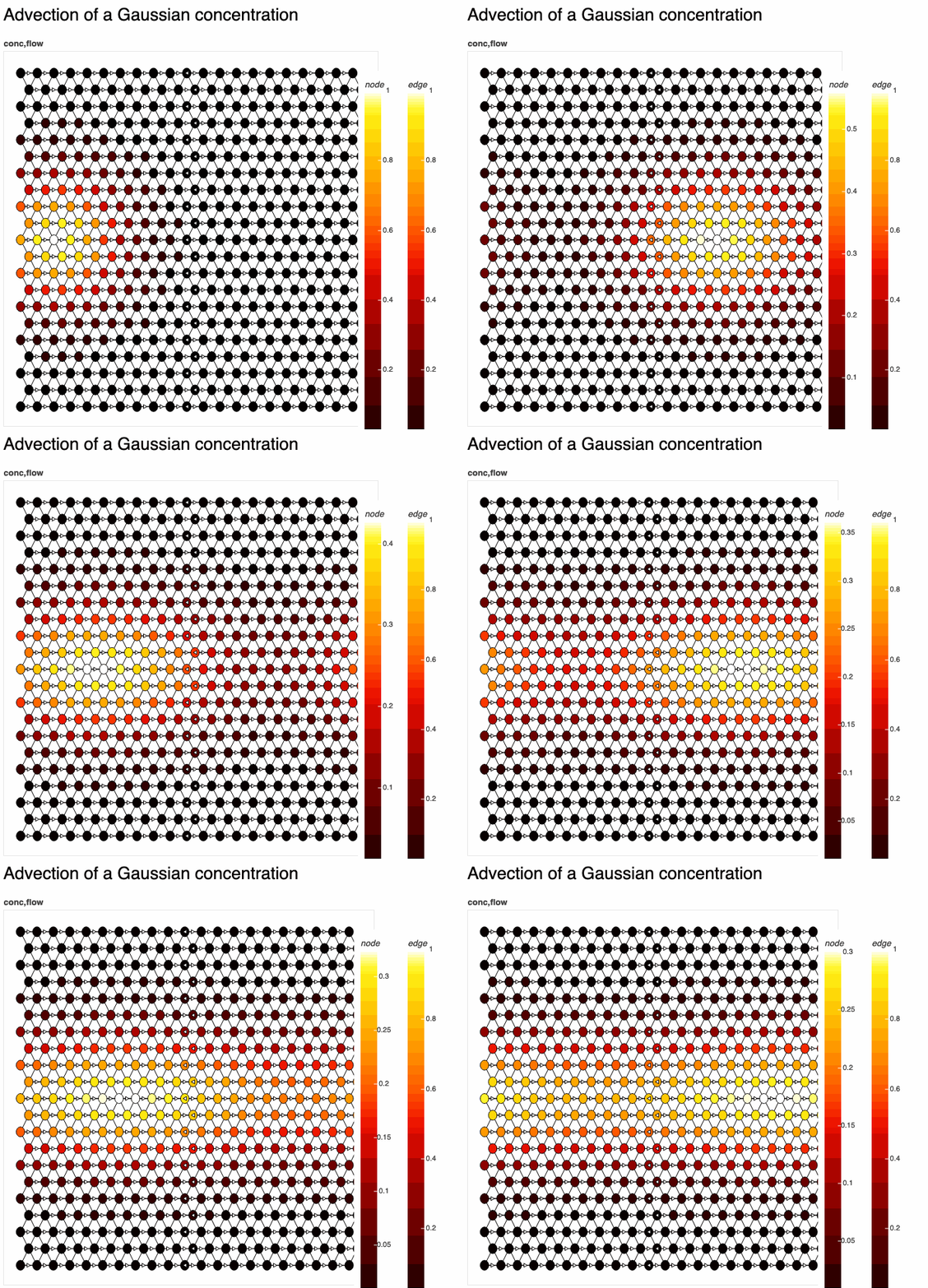
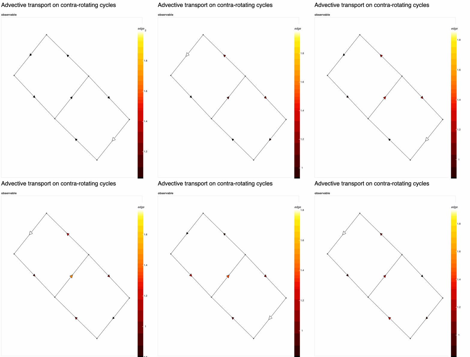
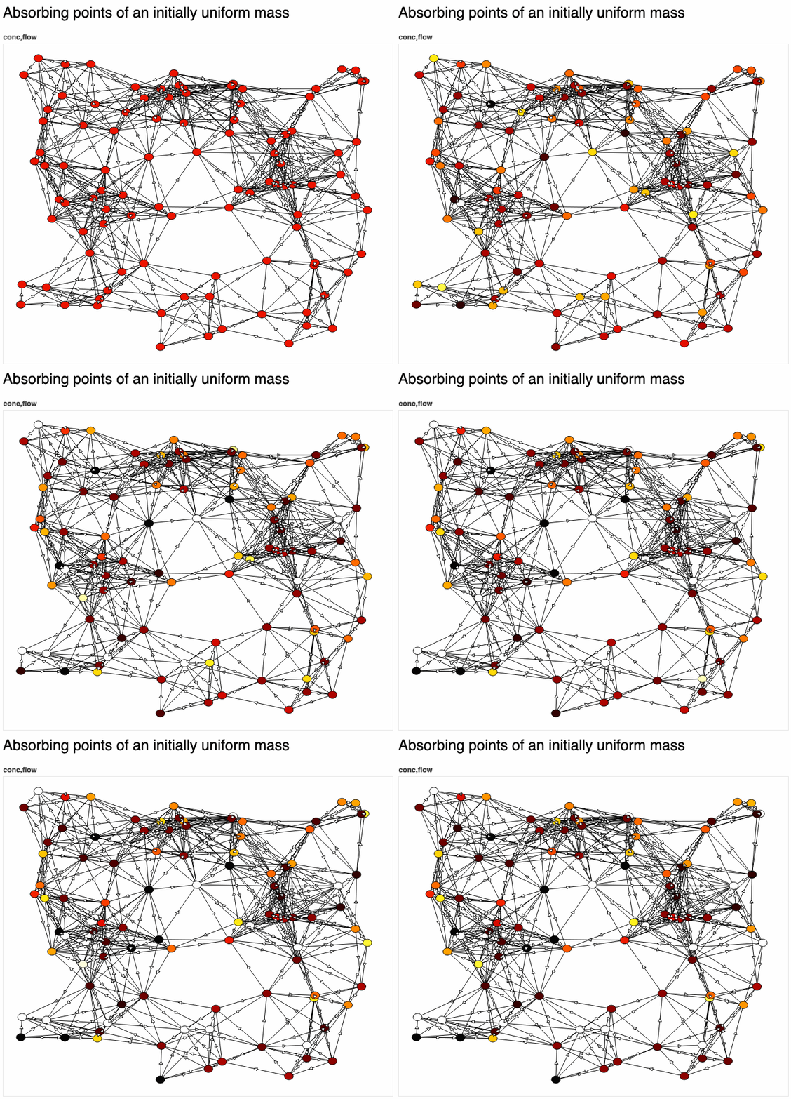
Simulate discrete- and continuous-time dynamics on networks, including PDEs, coupled map lattices, generalized cellular automata, and more.
Explore the docs [coming soon]»
- Built directly on top of NetworkX; represent observables (currently) on vertices or edges
- Spatial differential operators (gradient, divergence, laplace, advection) can be used in evolution laws, with more coming soon
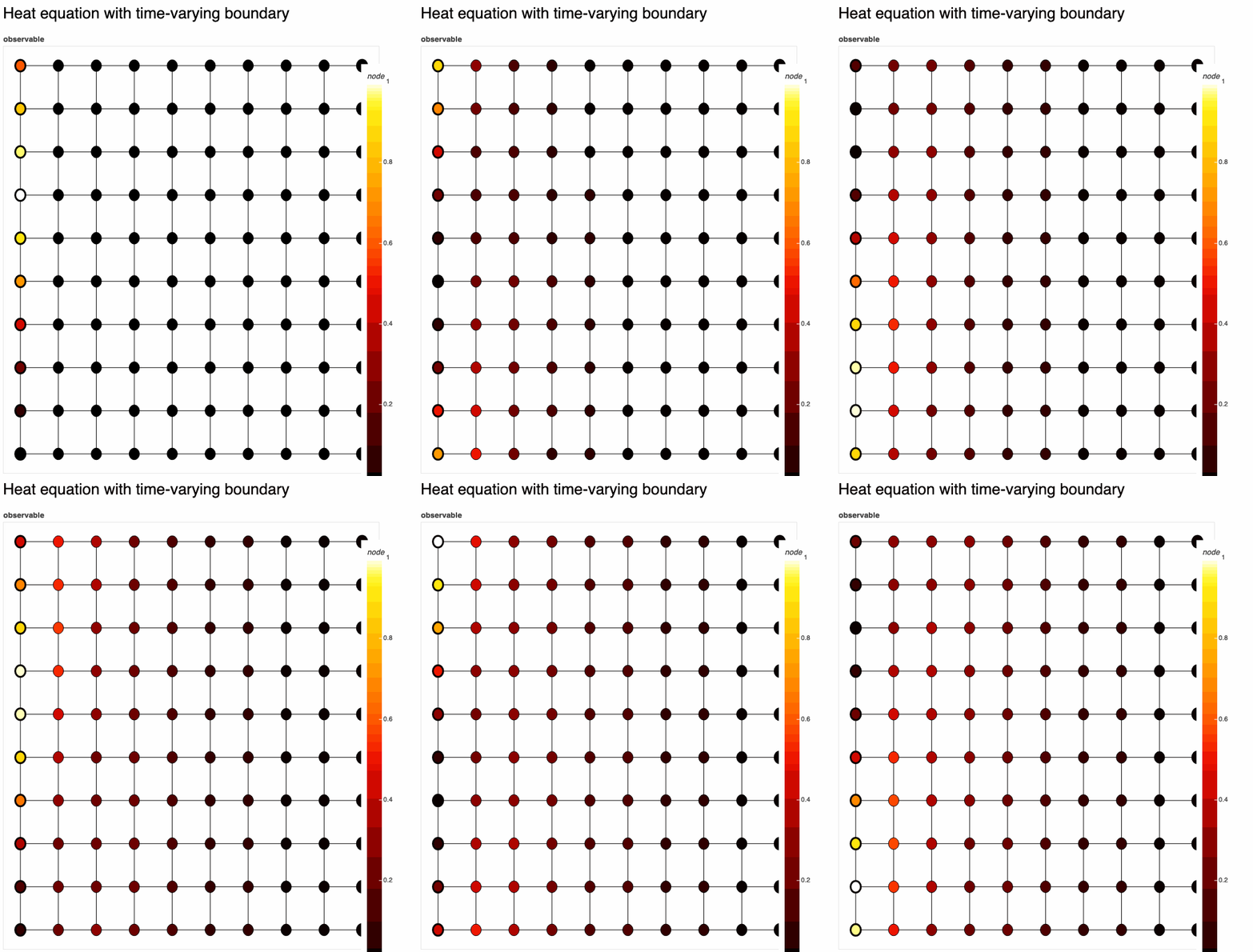
- Support for time-varying Dirichlet and Neumann boundary conditions
- Support for kinematic equations of motion via CVXPY
- Couple multiple discrete- or continuous-time observables across distinct graphs
- Automatic calculation of Lyapunov spectra using PyTorch and jax
As well as in-browser interactive rendering with Bokeh.
To get a local copy up and running follow these simple steps.
conda(recommended) or python >= 3.7
This has not been tested in all environments (especially Windows), so please report bugs.
- In local environment
pip install git+git://github.com/asrvsn/gds.git- As a project dependency
# Add to `requirements.txt`
-e git://github.com/asrvsn/gds.git#egg=gdsFor more examples, please refer to the Documentation (coming soon)
To start, import the library and define a graph:
import gds
import networkx as nx

G = nx.Graph() # Add nodes and edges
gds accepts any networkx.Graph object.
Dynamical systems in gds are scalar-valued functions defined over a particular graph domain, or fields. Typically we will use nodes or edges:
from gds import GraphDomain

# Suppose we want to define hydrodynamic equations
pressure = gds.node_gds(G)
velocity = gds.edge_gds(G)

assert (pressure.domain == GraphDomain.nodes)
assert (len(pressure.y) == len(G.nodes()))
assert (velocity.domain == GraphDomain.edges)
assert (len(velocity.y) == len(G.edges()))
These are simply |V|- and |E|-dimensional real-valued dynamical systems, constructed by some convenience functions node_gds, edge_gds.
However, in general we can define dynamical systems on k-simplices of G, which allows one to define dynamical systems on triangles, tetrahedra, and so on.
# Dynamics on k-simplices, or (k+1)-cliques, of G
k = 2
observable = gds.simplex_gds(k, G)We have observables on G, and now we must specify how they evolve. gds supports four types of evolution laws, and we'll use the heat equation to demonstrate each one. Start with
temperature = gds.node_gds(G)to define an observable, temperature, as a vertex field.
Specify the right-hand side of a differential equation.
# Continuous-time heat equation
temperature.set_evolution(dydt=lambda t, y: temperature.laplacian())
Various spatial differential operators, e.g. .laplacian(), are accessible as class methods of observables.
Specify the left-hand side of an algebraic equation equal to 0.
# Steady-state heat equation (aka Laplace equation)
temperature.set_evolution(lhs=lambda t, y: temperature.laplacian())Specify a map from a previous state to the next state.
temperature.set_evolution(map_fun=lambda t, y: y + temperature.laplacian())Specify a dataset to play back as an observable.
traj_t = np.linspace(0, 10, 100)
traj_y = np.zeros((len(G.nodes()), 100))
temperature.set_evolution(traj_t=traj_t, traj_y=traj_y)
This can be useful for "stitching" together data from previous runs with dependent variables, or for applying pre-defined control inputs.
Often, when expressing PDEs or ordinary differential equations, it's necessary or desired to impose boundary / initial conditions. gds makes expressing IBVPs easy using two methods:
# Initial conditions
temperature.set_initial(t0=0., y0=lambda x: 1. if x == my_special_node else 0.)
and
# Boundary conditions -- both time-varying and time-invariant, determined by function signature
temperature.set_constraints(dirichlet=gds.combine_bcs(
  lambda x: 0 if x[0] == 0 else None,
  lambda t, x: np.sin(t+x[1]/4)**2 if x[0] == 9 else None
))

# Boundary conditions -- Neumann conditions supported too
def neumann(t, x):
    if x[1] == n-1 and x[0] not in (0, n-1):
      return -0.1
    return None
temp.set_constraints(neumann=neumann)
Boundary conditions can be expressed in three ways:
- As a dictionary mapping points in space to values
- As a callable function of space
- As a callable function of time & space
gds will detect the type automatically, and all three types can be combined using gds.combine_bcs(). Time-invariant conditions will only be evaluated once.
Let's put it all together:
Definition:
G = gds.square_lattice(10, 10)
temperature = gds.node_gds(G)
temperature.set_evolution(dydt=lambda t, y: temperature.laplacian())
temperature.set_constraints(dirichlet=gds.combine_bcs(
  lambda x: 0 if x[0] == 9 else None,
  lambda t, x: np.sin(t+x[1]/4)**2 if x[0] == 0 else None
))
gds.render(temperature, title='Heat equation with time-varying boundary')
Here we have used gds.render(), which solves & renders temperature in real-time to a bokeh plot. There are many options for rendering. The result:
def navier_stokes(G: nx.Graph, viscosity=1e-3, density=1.0, inlets=[], outlets=[], **kwargs) -> (gds.node_gds, gds.edge_gds):
  '''
  G: graph
  '''
  pressure = gds.node_gds(G, **kwargs)
  velocity = gds.edge_gds(G, **kwargs)
  non_div_free = np.array([pressure.X[x] for x in set(inlets) | set(outlets)], dtype=np.intp)
  min_step = 1e-3

  def pressure_f(t, y):
    dt = max(min_step, velocity.dt)
    lhs = velocity.div(velocity.y/dt - velocity.advect()) + pressure.laplacian(velocity.div()) * viscosity/density
    lhs[non_div_free] = 0.
    lhs -= pressure.laplacian(y)/density
    return lhs

  def velocity_f(t, y):
    return -velocity.advect() - pressure.grad()/density + velocity.laplacian() * viscosity/density

  pressure.set_evolution(lhs=pressure_f)
  velocity.set_evolution(dydt=velocity_f)

  return pressure, velocity
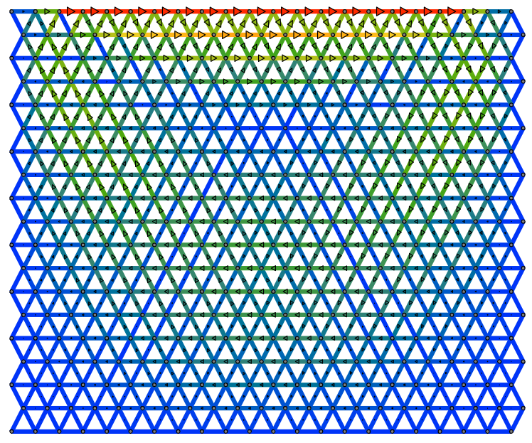
Lid-driven cavity on a triangular lattice:
def SIR_model(G,
    dS=0.1, dI=0.5, dR=0.0,   # Diffusive terms
    muS=0.1, muI=0.3, muR=0.1,  # Death rates
    Lambda=0.5,         # Birth rate
    beta=0.2,           # Rate of contact
    gamma=0.2,          # Rate of recovery
    initial_population=100,
    patient_zero=None,
    **kwargs):
  '''
  Reaction-Diffusion SIR model
  Based on Huang et al, https://www.researchgate.net/publication/281739911_The_reaction-diffusion_system_for_an_SIR_epidemic_model_with_a_free_boundary
  '''
  susceptible = gds.node_gds(G, **kwargs)
  infected = gds.node_gds(G, **kwargs)
  recovered = gds.node_gds(G, **kwargs)

  susceptible.set_evolution(dydt=lambda t, y:
    dS*susceptible.laplacian() - muS*susceptible.y - beta*susceptible.y*infected.y + Lambda
  )

  infected.set_evolution(dydt=lambda t, y:
    dI*infected.laplacian() + beta*susceptible.y*infected.y - muI*infected.y - gamma*infected.y
  )

  recovered.set_evolution(dydt=lambda t, y:
    dR*recovered.laplacian() + gamma*infected.y - muR*recovered.y
  )

  if patient_zero is None:
    patient_zero = random.choice(list(G.nodes()))
  print(patient_zero)
  susceptible.set_initial(y0=lambda x: initial_population)
  infected.set_initial(y0=lambda x: 1 if x == patient_zero else 0.)

  sys = gds.couple({
    'Susceptible': susceptible,
    'Infected': infected,
    'Recovered': recovered
  })

  return sys
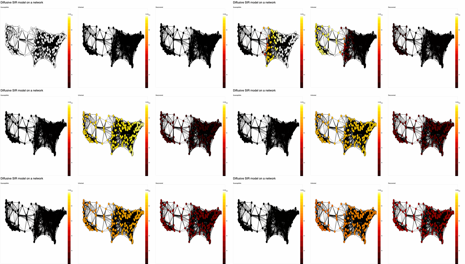
Zero-flux SIR model with R0=2:
[Note: this assumes diffusive spread only via geographical shortest paths.]
G = gds.square_lattice(10, 10)
temperature, velocity_x, velocity_y = gds.node_gds(G), gds.node_gds(G), gds.node_gds(G)
More examples are coming soon.
See the open issues for a list of proposed features (and known issues).
- Detailed docs
- Lyapunov exponent calculation for continuous-time dynamics
- Probabilistic cellular automata
- Full support for k-simplex dynamical systems
Distributed under the MIT License. See LICENSE for more information.
