savvi is a package for Safe Anytime Valid Inference. Also, it’s a savvy pun.
From Ramdas et al. (2023):
Safe anytime-valid inference (SAVI) provides measures of statistical evidence and certainty – e-processes for testing and confidence sequences for estimation – that remain valid at all stopping times, accommodating continuous monitoring and analysis of accumulating data and optional stopping or continuation for any reason.
pip install git+https://github.com/assuncaolfi/savviFor development, use pdm.
Implementation of tests from Anytime-Valid Inference for Multinomial Count Data (Lindon and Malek 2022). Application examples were also adapted from the same publication.
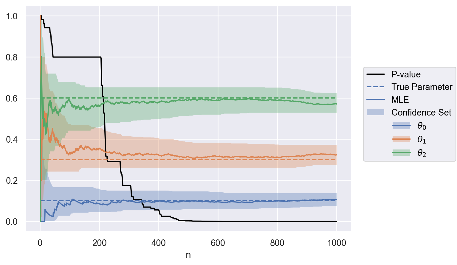
Application: sample ratio mismatch.
Consider a new experimental unit
import numpy as np

np.random.seed(1)
theta = np.array([0.1, 0.3, 0.6])
size = 1000
xs = np.random.multinomial(1, theta, size=size)
print(xs)
[[0 1 0]
[0 0 1]
[0 0 1]
...
[0 1 0]
[1 0 0]
[0 0 1]]
We can test the hypothesis
with
from savvi import Multinomial

u = 0.05
theta_0 = np.array([0.1, 0.4, 0.5])
test = Multinomial(0.05, theta_0)
For each new unit sample
import cvxpy as cp


def run_sequence(test, xs, **kwargs):
    size = xs.shape[0]
    sequence = [None] * size
    stop = np.inf
    for n, x in enumerate(xs):
        test.update(x, **kwargs)
        sequence[n] = {
            "n": test.n,
            "p": test.p,
            "mle": test.mle.tolist(),
            "confidence_set": test.confidence_set.tolist(),
        }
        if test.p <= u:
            stop = min(stop, n)
    optional_stop = sequence[stop]
    return sequence, optional_stop


solver = cp.CLARABEL
sequence, optional_stop = run_sequence(test, xs, solver=solver)
optional_stop
{'n': 402,
'p': 0.04845591105969517,
'mle': [0.09950248756218906, 0.3208955223880597, 0.5796019900497512],
'confidence_set': [[0.056684768115202705, 0.1493967591525672],
[0.2608987241982874, 0.4028302603098119],
[0.4971209299792429, 0.6517617329309116]]}
Code
import polars as pl
import seaborn.objects as so


def to_df(sequence, parameter, value):
    size = len(sequence)
    data = (
        pl.from_dicts(sequence)
        .explode("confidence_set", "mle")
        .with_columns(
            confidence_set=pl.col("confidence_set").list.to_struct(
                fields=["lower", "upper"]
            ),
            parameter=pl.Series(parameter * size),
            value=pl.Series(value.tolist() * size),
        )
        .unnest("confidence_set")
    )
    return data


def plot(data):
    plot = (
        so.Plot(data.to_pandas(), x="n")
        .add(so.Line(color="black"), y="p", label="P-value")
        .add(so.Line(linestyle="dashed"), y="value", color="parameter", label="True Parameter")
        .add(so.Line(), y="mle", color="parameter", label="MLE")
        .add(
            so.Band(alpha=1 / theta.size),
            ymin="lower", ymax="upper", color="parameter", label="Confidence Set"
        )
        .label(color="", y="")
        .limit(y=(-0.05, 1.05))
    )
    return plot


parameter = [f"$\\theta_{i}$" for i in np.arange(0, theta.size)]
data = to_df(sequence, parameter, theta)
plot(data)
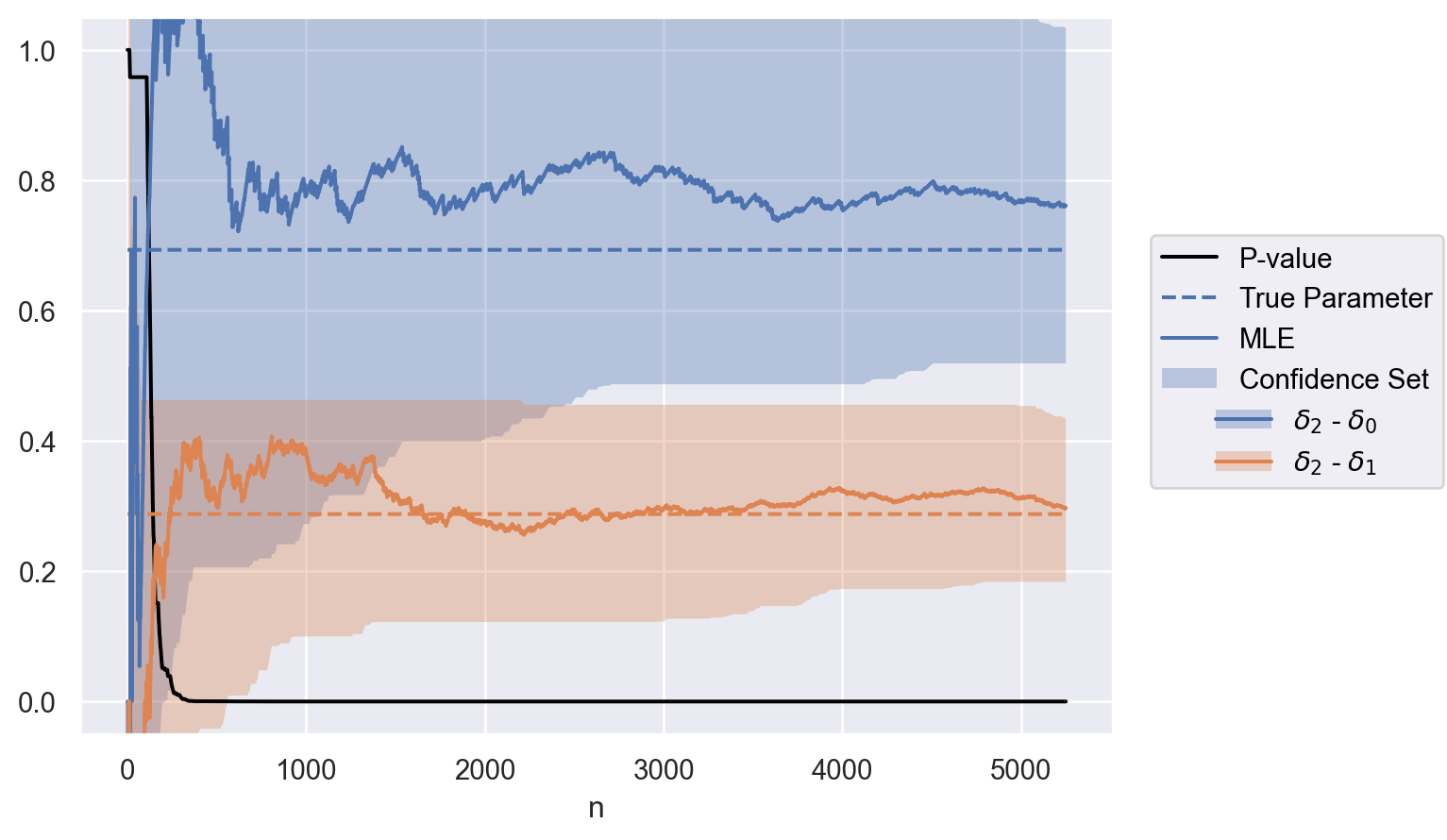
Application: conversion rate optimization when all groups share a common multiplicative time-varying effect.
Suppose a new experimental unit
Therefore, the next Bernoulli success comes from a random group,
rho = np.array([0.1, 0.3, 0.6])
delta = np.log([0.2, 0.3, 0.4])
theta = rho * np.exp(delta) / np.sum(rho * np.exp(delta))
size = 5250
xs = np.random.multinomial(1, theta, size=size)
print(xs)
[[0 1 0]
[0 1 0]
[0 1 0]
...
[0 0 1]
[0 0 1]
[0 0 1]]
We can test the hypothesis
using a Multinomial test with
test = Multinomial(u, rho)
test.hypothesis = [
    test.delta[0] >= test.delta[1],
    test.delta[0] >= test.delta[2],
]
We can also set contrast weights
test.weights = np.array([[-1, 0, 1], [0, -1, 1]])For each new unit sample
sequence, optional_stop = run_sequence(test, xs, solver=solver)
optional_stop
{'n': 210,
'p': 0.04861129531258319,
'mle': [1.0986122886681098, 0.21622310846963605],
'confidence_set': [[0.0020567122072947704, 1.4880052569753974],
[-0.3216759113208812, 0.4627565948192972]]}
Code
parameter = ["$\\delta_2$ - $\\delta_0$", "$\\delta_2$ - $\\delta_1$"]
contrasts = test.weights @ delta
data = to_df(sequence, parameter, contrasts)
plot(data)
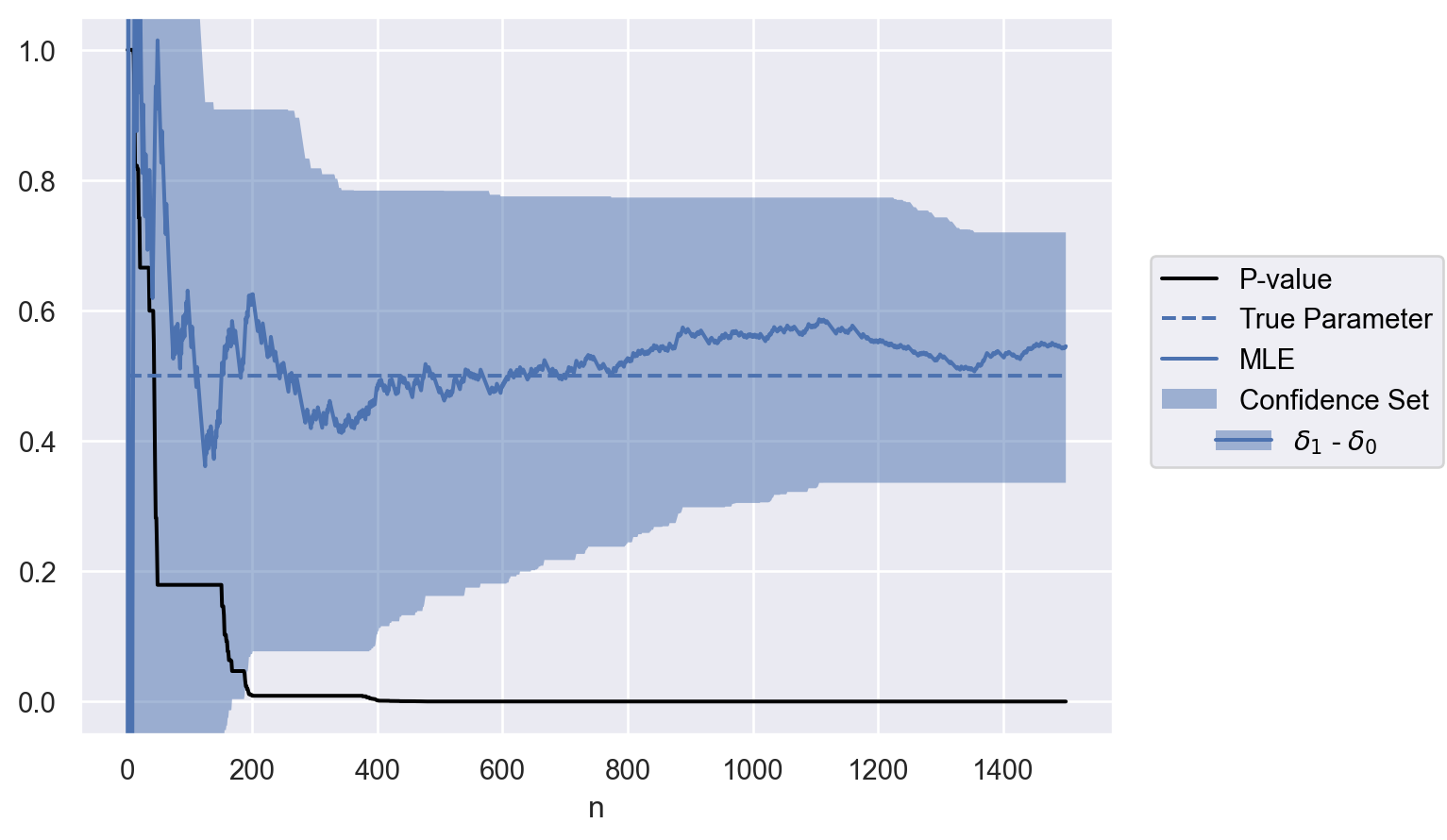
Application: software canary testing when all processes share a common multiplicative time-varying effect.
Consider points are observed from one of
Therefore, the next point comes from a random process, distributed as
rho = np.array([0.8, 0.2])
delta = np.array([1.5, 2])
theta = rho * np.exp(delta) / np.sum(rho * np.exp(delta))
size = 1500
xs = np.random.multinomial(1, theta, size=size)
print(xs)
[[1 0]
[0 1]
[1 0]
...
[0 1]
[1 0]
[0 1]]
We can test the hypothesis
using a Multinomial test with
test = Multinomial(u, rho)We can also set contrast weights
test.weights = np.array([[-1, 1]])For each new unit sample
sequence, optional_stop = run_sequence(test, xs, solver=solver)
optional_stop
{'n': 168,
'p': 0.04675270375081281,
'mle': [0.5839478885949534],
'confidence_set': [[0.0036592933902448955, 0.9085292981365327]]}
Code
parameter = ["$\\delta_1$ - $\\delta_0$"]
contrasts = test.weights @ delta
data = to_df(sequence, parameter, contrasts)
plot(data)
Lindon, Michael, and Alan Malek. 2022. “Anytime-Valid Inference for Multinomial Count Data.” In Advances in Neural Information Processing Systems, edited by Alice H. Oh, Alekh Agarwal, Danielle Belgrave, and Kyunghyun Cho. https://openreview.net/forum?id=a4zg0jiuVi.
Ramdas, Aaditya, Peter Grünwald, Vladimir Vovk, and Glenn Shafer. 2023. “Game-Theoretic Statistics and Safe Anytime-Valid Inference.” https://arxiv.org/abs/2210.01948.


