MapMatching4GMNS

Please send your comments to xzhou74@asu.edu if you have any suggestions and questions.

A work-in-progress user guide can be found at

User Guide of Trace2Route_v3 - Google Docs

1. Introduction

Based on input network and given GPS trajectory data, the map-matching program of MapMatching4GMNS (trace2route.exe) aims to find the most likely route in terms of node sequence in the underlying network, with the following data flow chart.

GMNS: General Modeling Network Specification (GMNS) (https://github.com/zephyr-data-specs/GMNS)

2. Data flow

	files	Data Source	Visualization
GMNS network input	node.csv, link.csv	Openstreetmap	QGIS, web interface for GMNS
Location sequence data input	trace.csv	GPS traces downloaded from OpenStreetMap, e.g., using the script at https://github.com/asu-trans-ai-lab/MapMatching4GMNS/blob/master/release/get_gps_trace.py	QGIS
Map-matched output	route.csv		QGIS

Windows Executable: trace2route.exe can be found from

https://github.com/asu-trans-ai-lab/MapMatching4GMNS/tree/master/release

3. File description

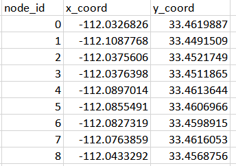
File node.csv gives essential node information of the underlying network in GMNS format, including node_id, x_coord and y_coord.

File link.csv should include essential link information of the underlying (subarea) network, including from_node_id, to_node_id, length and geometry.

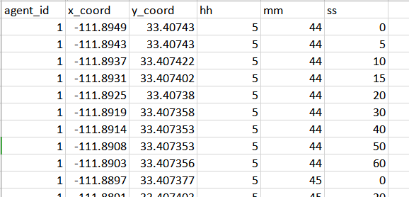
Input trace file as

The agent id is GPS trace id, x_coord and y_coord should be consistent to the network coordinate defined in node.csv and link.cvs. Fields hh mm and ss correspond the hour, minute and second for the related GPS timestamp. We use separate columns directly to avoid confusion caused by different time coding formats.

Please note that, for mapping applications such as mapping sensor TMC corridors to the planning network, mapping bus lines to the highway driving network, the fields of hh, mm, ss are not needed. But we need to specify the origin node (identified by the first coordinate point) clearly so that the most likely path algorithm can be correctly performed.

Output file description

File route.csv describes the most-likely path for each agent based on input trajectories.

4. Visualization

Step 1: Load GMNS files in QGIS

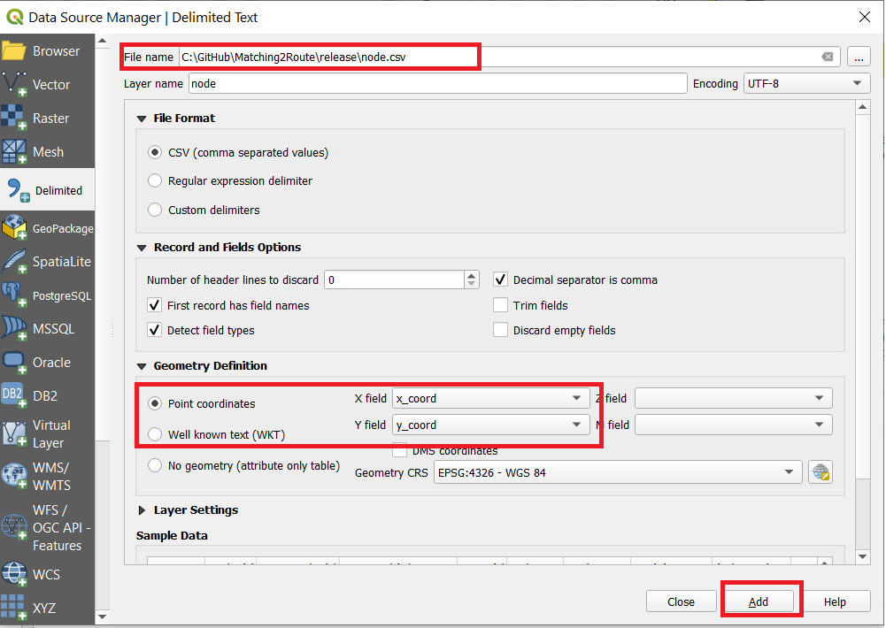
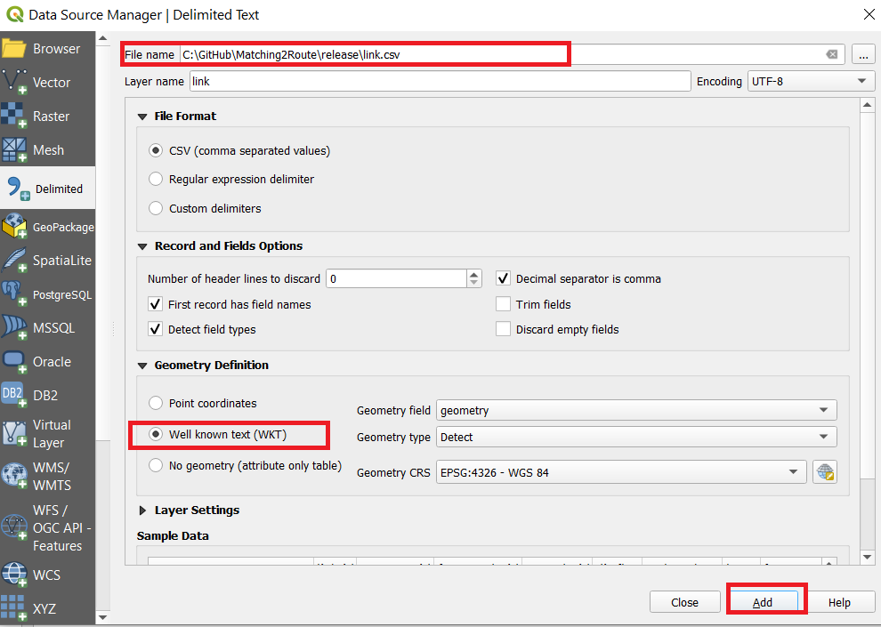
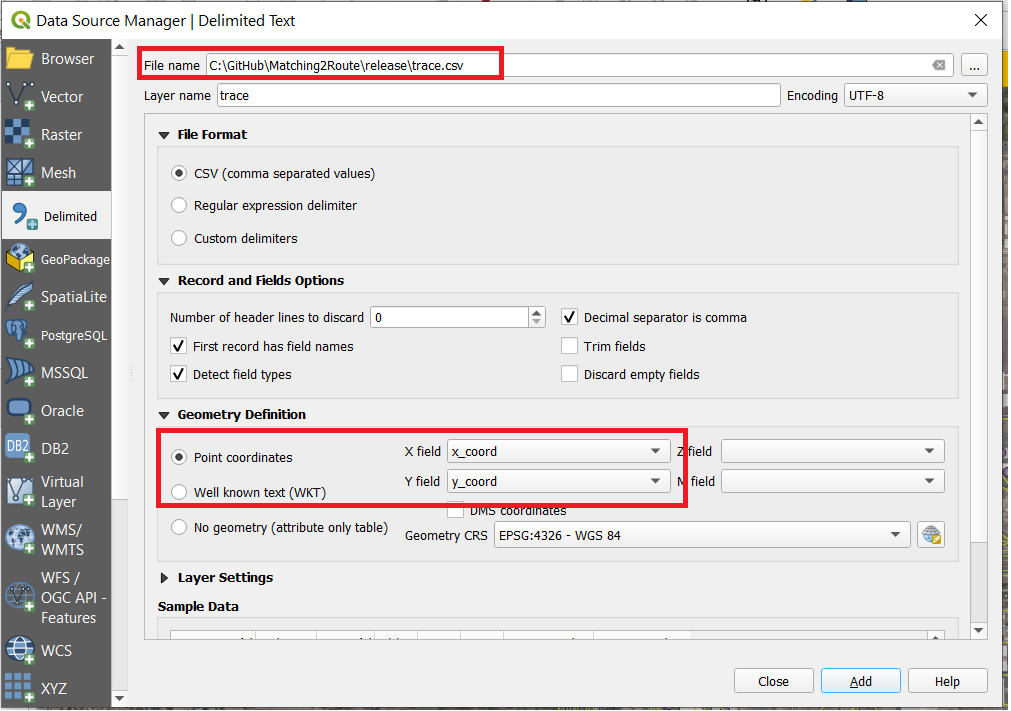
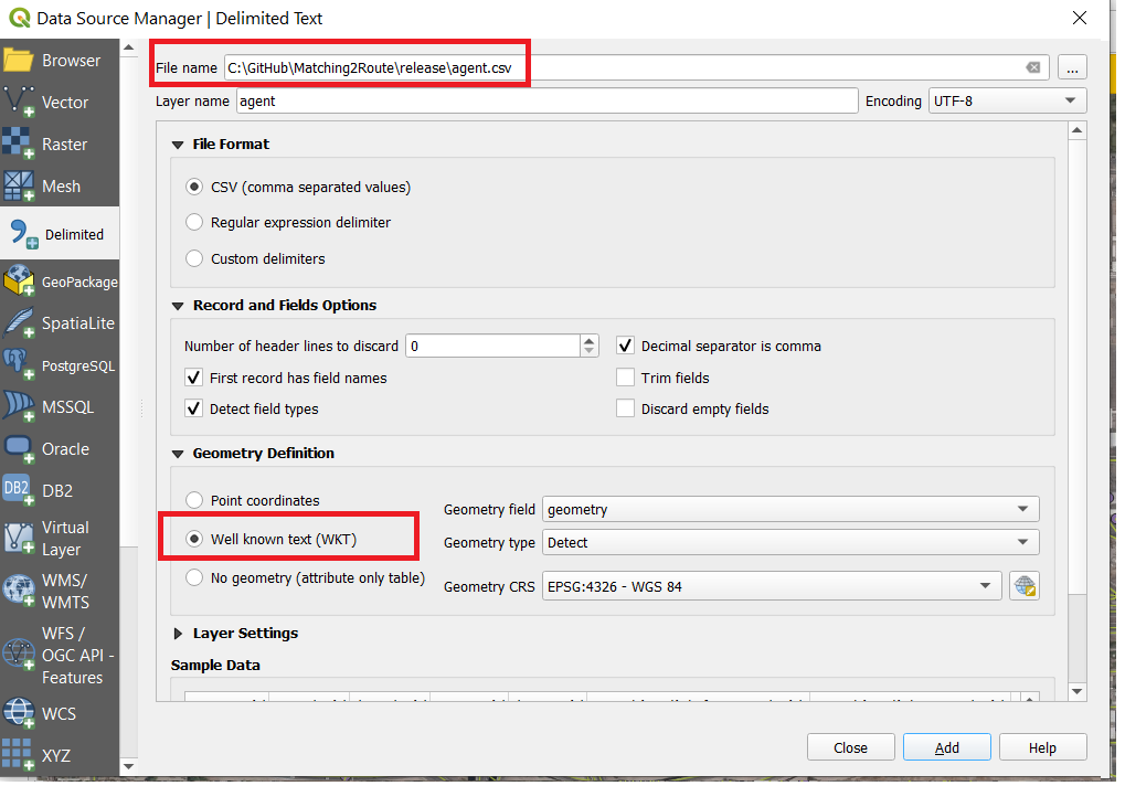
Install and open QGIS and click on menu Layer->Add->Add Delimited Text Layer. In the following dialogue box, load GMNS node.csv and link.csv, and ensure
“point coordinates” is selected as geometry definition for node.csv wit x_coord and y_coord for “Geometry field”, and WKT is selected as geometry definition for link.csv.

Step 2: Load XYZ Tiles in QGIS with background maps

Find XYZ Tiles and double-click OpenStreetMap on Browser panel. Please move the background layer to the bottom to show the GMNS network.

Refence: https://gis.stackexchange.com/questions/20191/adding-basemaps-from-google-or-bing-in-qgis

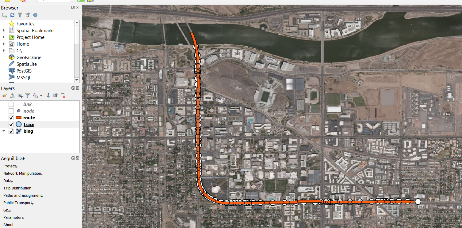
Step 3. Visualize input trace and output route files in QGIS

The 'geometry' field can be obtained from link.csv file. Then open this file in the same way as above. (Menu Layer->Add->Add Delimited Text Layer)

5. Algorithm

Read standard GMNS network files node and link files, Read GPS trace.csv file
Note: the TRACE2ROUTE program will convert trace.csv to input_agent.csv for visualization in NeXTA.
Construct 2d grid system to speed up the indexing of GSP points to the network. For example, a 10x10 grid for a network of 100 K nodes could lead to 1K nodes in each cell.
Identify the related subarea for the traversed cells by each GPS trace, so only a small subset of the network will be loaded in the resulting shortest path algorithm.
Identify the origin and destination nodes in the grid for each GPS trace, in case, the GPS trace does not start from or end at a node inside the network (in this case, the boundary origin and destination nodes will be identified). The OD node identification is important to run the following shortest path algorithm.
Estimate link cost to calculate a generalized weight/cost for each link in the cell, that is, the distance from nearly GPS points to a link inside the cell.
Use likely path finding algorithm selects the least cost path with the smallest generalized cumulative cost from the beginning to the end of the GPS trace.
Identify matched timestamps of each node in the likely path
Output route.csv with estimated link travel time and delay based on free-flow travel time of each link along the GPS matched routes

Reference

This code is implemented partially based on a published paper in Transportation Research Part C:

Tang J, Song Y, Miller HJ, Zhou X (2015) “Estimating the most likely space–time paths, dwell times and path uncertainties from vehicle trajectory data: A time geographic method,” Transportation Research Part C, http://dx.doi.org/10.1016/j.trc.2015.08.014