This is reinforced-scinet, learning operationally meaningful representations of
reinforcement learning (RL) environments.
This code accompanies our paper,
H. Poulsen Nautrup, T. Metger, R. Iten, S. Jerbi, L.M. Trenkwalder, H. Wilming, H.J. Briegel and R. Renner
Operationally meaningful representations of physical systems in neural networks,
arXiv:2001.00593 [quant-ph] (2020).
If you use any of the code, please cite our paper. Here, we provide the PyTorch code for the examples from Sec. 6 of the paper and beyond. In particular, this repository contains:
- Code for asynchronous RL with deep energy-based projective simulation models.
- Code for asynchronous representation learning as described in the paper.
- Trained models along with detailed results from the evaluation of the model.
The code for the examples that do not involve RL can be found here.
Enjoy!
In order to run the code you will require the following:
python 3.7.4numpy 1.17.2torch 1.2.0matplotlib 3.1.1gym-subgridworld 0.0.2from here
You may run the code with different versions, but these are the versions we have verified the code with. We also recommend working with GPU since we have not thoroughly tested the code with only CPUs.
There is quite a lot of documentation in the code already. For further questions, please contact us directly.
The asynchronous architecture is inspired by GA3C.
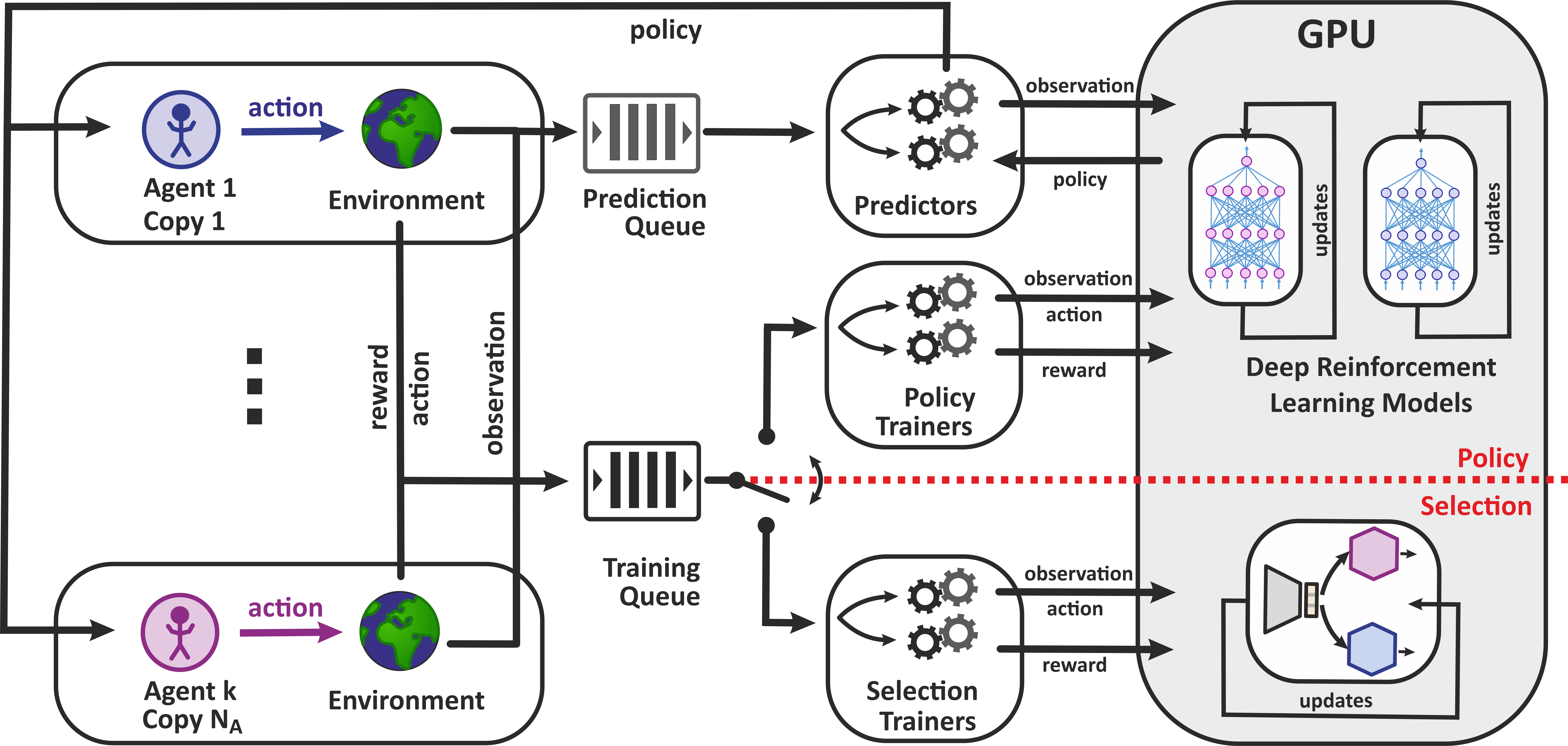
In policy mode we train various deep energy-based projective simulation (DPS) models on the same environment
but with different objectives.
In selection mode we use neural networks to encode and decode observations received from a RL environment.
The decoders either predict the behavior of trained RL agents or reproduce the observation like an autoencoder.
The architecture is designed to be asynchronous and may make use of a GPU. A more detailed description can be found
in the paper.
The specific architecture can be illustrated as follows:
You can immediately run the code to predict the behavior of three trained deep reinforcement learning models. To this end, you just need to run the main.py file with python and watch the results being logged to your console. (You might have to move the content of data/publication/ to data/ so it can be loaded.)
Chances are that your local computer cannot run the code with the same parameters that we used.
You can decrease the workload by reducing the number of processes in the config.py.
That is, you need to lower the numbers of WORKERS, TRAINERS and PREDICTORS.
For example, you can try 8 workers, 1 trainer and 1 predictor for each environment ID.
If you cannot use a GPU, you can change the DEVICE parameter to cpu. However, we have not thoroughly tested this.
Once you run the program, you should see numbers like the following:
[ Training #       34400 ][ Episode #     341 ][ Loss for type: Policy ][ Trainer for type:  env1 ][ Loss: 1.20120335. ]
[ Training #       34400 ][ Episode #     342 ][ Loss for type: Autoencoder ][ Trainer for type:  env1 ][ Loss: 0.29708305. ]
What you see is the training of the prediction agents and an autoencoder. Given an environment objective (here env1), the policy prediction has a smooth L1 loss of 1.2. The autoencoder trying to reproduce the input has a binary cross entropy loss of 0.2 97. Over time, this will be reduced while the selection neurons start affecting the latent representation with noise. A log of the amount of noise is being generated at results_log/selection.txt. There you find results like this:
env1, [-9.83377456665039, -9.83377456665039, -9.83377456665039]
These numbers quantify the noise of the three selection neurons for the environment objective (or decoder agent) env1. Once one of these values increases above 0. the value of the associated latent neuron cannot be recovered by a decoder.
In the paper, we demonstrate representation learning for a sub-grid world environment. Here, we describe how you may reproduce those results. The code for the environment can be found here.
As described above, we split the training into two modes.
In this training mode, we train the DPS agents on the RL environment.
For the results, we first trained three DPS agents to solve the sub-grid world environment.
The parameters can be found in the config.py file. In order to reproduce the results, you need to switch TRAIN_MODE
from selection to policy mode, set LOAD_PS to False for all agents, and run the main.py for 3M episodes.
For your convenience, we already provide the pretrained agents in the load_models folder. When training these agents,
they performed as follows:
In this training mode, we train decoders to predict behavior of DPS agents or reproduce the input.
This is the current setting of the code and can be immediately performed by running bash _run.sh or python main.py
in the main directory.
That is, if you run the code as is, you will start training one autoencoder and three decoders to predict the behavior
of the pretrained DPS agents.
At the same, selection neurons will pressure the encoder to create a representation of the observation that can be
shared among decoders efficiently.
In obtaining the results in the paper, we observed the following loss:


