ATMS 523 Weather and Climate Data Analytics
Module 4: Time Series and EOF Analysis
In this module we will learn:
- how to work with
stasmodel - how to work and interpret
eofsfunction
There are 6 problems that need to be done to complete this module. The hints for the problems can be found in this work: (https://climate.usu.edu/people/yoshi/pyclm101/monthly.html)
1. Create Dataset for monthly mean SST and Precipitation anomalies
Here I used both sea surface temperature and precipitation dataset from RDA NCAR with code ds633.1. However, for the precipitation dataset, it is not direct acummulated precipiattion with milimiter (mm) units, it is the sum of large and convective precipitation flux. So, the unit is in kg m/s^2.
To get the anomalies, I simply subtstracted the monthly mean with its monthly mean average. Though the original data is in Kelvin unit, but after subtracting, we can also consider that the anomalies is in Celcius unit (there is no different on Kelvin and Celcius for value difference). After that I save those anomalies dataset on my local computer so that it will ease the next process as we do not need to access the dataset from the original website (which is sometimes not accessible due to maintainence issue).
However, due to the the size limitation buth anomalies dataset were not uploaded in this github.
2. Apply the statistical processing (deasasonal, detrend, and standardization)
This problem is actually preparing us to calculate EOF component of our SST anomalies dataset. There are three steps (shown below) to complete the statistical processing.
- Deseasonal is a way to drop a distinct pattern in the dataset, especially if there is a repition pattern over some interval range. This can be yearly, monthly, seasonlity, daily, or hourly.
- Detrend is a process to remove the increasing/decreasing pattern found in dataset so that after we applied the detrend step, the data will be stationer.
- Standardization is an attempt to have same standard deviation so taht in the end the data will have same range value.
3. Perform an EOF analysis with respect on cosine latitude weighting and plot the first 5 EOFs
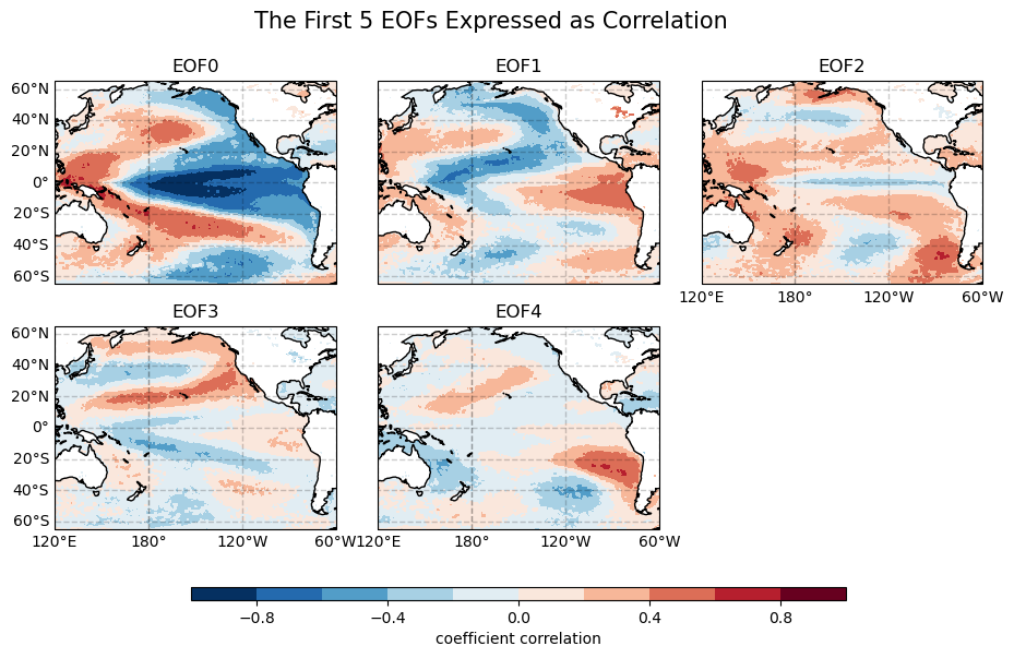
Here I aplied eofs package to answer the problem. Empirical Orthogonal Function (EOF) is a mathematical function defining the dominant modes by decomposing 3-dimensional dataset into spatial and time-series pattern. Though it is slightly different, we can also call EOF as Principal Componenet Analysis (PCA). For this problem I set the number of EOF mode 10, and then only plot the first-5 EOF modes as correlation to see the relationship between each mode to original SST anomalies dataset.
Here we can see that each mode shows different signal in Pacific (Nino 3.4 area). But, the first EOFs diplayed more clear signal of correlation than others.
4. Plot the percentage of variance exolained by the first 10 EOFs.
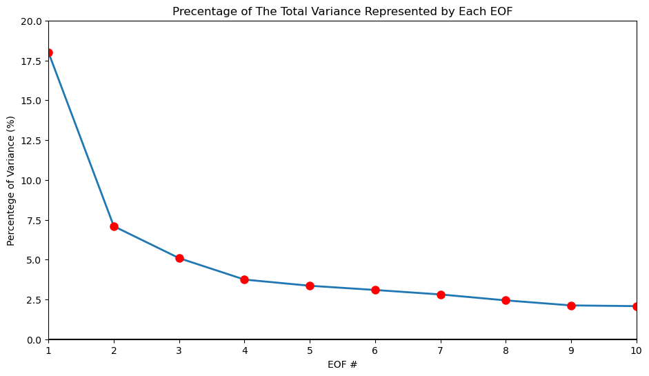
From the percantage variance we know that the first EOF mode can explain more tahn 17.5% variance in the data. Then the precentage decrease along the number.
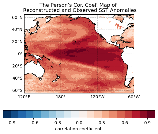
5. Reconstruct the first-5 EOFS to get the SST anomalies and plot a map of Person correlation between the reconstructed and observed SST anomalies.
From problem #4 we know that the first-5 EOFs mode has larger precentage variance, so that for this problem we only use those modes to reconstruct the SST anomalies.
We can see that the reconstructed SST anomalies with first-5 mode has strong correlation with the observed data. It has positive correlation with the central Nino3.4 hit > 0.9. We can say that the first-5 modes can explain the SST anomalies.
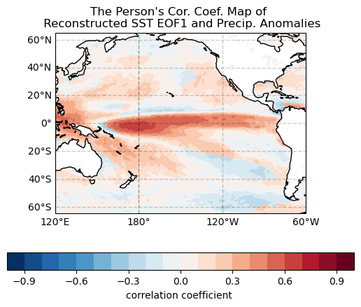
6. Plot a map of recontructed SST anomalies with precipitation anomalies dataset.
The above figure shows us that reconstruced SST anomalies has a strong positive correlation with precipitation number in Pacific, especially Nino3.4 area. We can say that the SST and precipitation anomalies somewhat display the signal of ENSO in the area.
Good Luck and Happy Sharing 😎
Reference 📄
- European Centre for Medium-Range Weather Forecasts. 2019, updated yearly. ERA5 Reanalysis (Monthly Mean 0.25 Degree Latitude-Longitude Grid). Research Data Archive at the National Center for Atmospheric Research, Computational and Information Systems Laboratory. https://doi.org/10.5065/P8GT-0R61. Accessed† 10-Oct-2022.
- EOF analysis https://climate.usu.edu/people/yoshi/pyclm101/monthly.html
- EOF package https://github.com/ajdawson/eofs
Copyright 📣
Full code can be found through this address: https://github.com/atmsillinois/time-series-and-eofs-fsari2/blob/main/HW04_Fitria.ipynb


