- Develop an end-to-end approach for a self-driving car in a simulated environment
- end-to-end means: The model gets camera images as input and controls the vehicle with the steering angle as output. No manual extraction of features or route planning needed. Similar to NVIDIA or comma.ai approach.
- Model must drive the car at least 1 round in track 1
- As challenge: Let the model drive the car in track 2
- Literature research:
- NVIDIAs paper on their approach
- Sentdex' Python Plays GTA V project.
- Siraj Raval' video on this topic
- Slack/Forum of Udacity
- Use the provided Udacity simulator to collect data of good driving behavior as training data
- Build a convolution neural network in Keras that predicts steering angles from images
- Train and validate the model with the training and validation set
- Test the models autonomous functionality in track 1 in the simulation and check if it behaves correctly
- Change network architecture and data pipeline if necessary
- Train and test the model in track 2
- Collect additional data of critical scenes if necessary
- Repeat until one model can drive the car in track 1 and track 2
My project includes the following files:
- model.py containing the script to create and train the model
- helper.py containing various helper functions used by model.py
- data_augmentation.py is an universal image augmentation functions, gets called by helper.py
- drive.py for driving the car in autonomous mode
- model.h5 containing a trained convolution neural network
- README.md summarizing the project
- car-view video of track 1 & 2 track1.mp4 & track2.mp4, same model
- link for my recorded data (mega.nz)
Using the Udacity provided simulator and the drive.py file, the car can be driven autonomously around the track by executing
python drive.py model.h5Python, Keras and all dependencies must be installed.
The model.py file contains the code for training and saving the convolution neural network. The file shows the pipeline for training the model, and it contains comments to explain how the code works.
Given and recorded data is each structered in a folder of images and a .csv-file (log), which contains all the links to the images as well as the steering angle and other information. Udacity provided a dataset with 24108 images (24108 / 3 perspectives = 8036 scene samples) for track 1, which was very helpful. They are 320 pixels wide * 160 pixels high and taken from 3 perspectives by virtual cameras (center, left, right).
Exploration of the dataset lead to the some observations:
- Simple and similar graphics, easy to learn but danger of overfitting.
- Track 1 is clockwise round track with almost all turns being left - unbalanced, left-biased dataset.
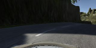
- Track 2 is very different looking, with lots of sharp bends and vertical up and downs. Also the occurrence of a lot of shadows could be problematic (see 2.2 examples of track 2). Developing a model to generalize and drive both tracks will be challenging
For track 1 17259 images (5753 samples) were acquired by using a joystick as input. Here I came across the first problem: Unity doesn't take the (Windows-)calibrated signals from a joystick, solution see here(forum). The acquired data contains 2 laps of track 1, also 2 in reverse and different critical scenes, like the bridge, the turn after the bridge,. etc. Folders are: me_data, me_data2, me_data3, me_data4
For track 2 43710 images (14570 samples) were acquired, this are 5 complete laps driving as near to the middle line as possible and some critical scenes extra. Folders are: me_track2_data, me_track2_data2, me_track2_data3
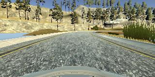
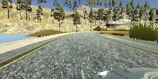
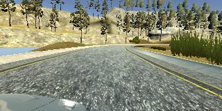
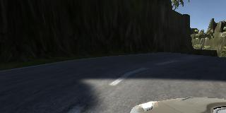
Example of a scene sample(center, left, right camera) of track 1:
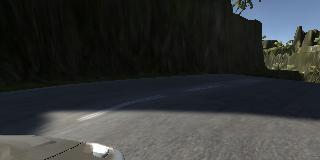
Example of track 2:
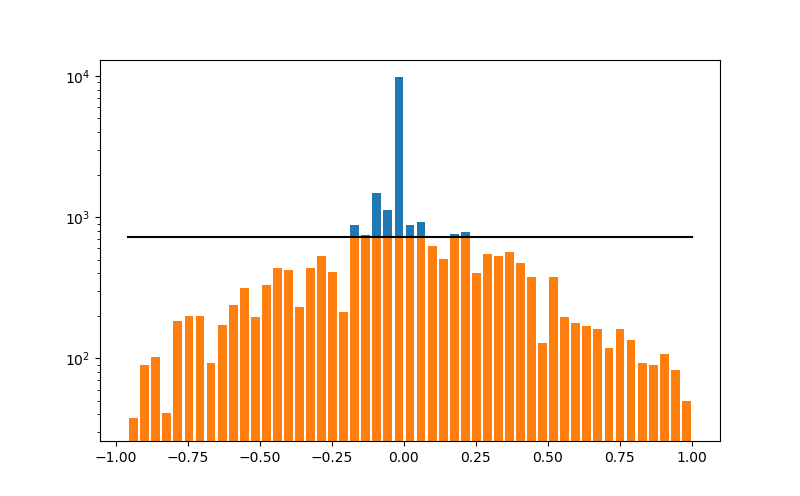
Most of the samples were driving straight which leads to a big bias for going straight. A function was implemented, which deletes as much sample as there are over a defined maximum in one bin. This maximum was defined as 1.3 times the mean as shown by the black line in the diagram below.
After the cleaning process 17433 samples were left.
The histogram shows:
- blue: distribution before cleaning,
- orange : distribution after cleaning.
To provide more data (more data is always better) without any recording and reduce shortcomings in the dataset, several data augmentation techniques were tried. This enables the extraction of more information which helps prevent overfitting and getting generalization. A general image augmentation function data_augmentation.py was implemented and used.
Used techniques (every technique outputs new images):
-
Flip (np.fliplr) the image and mupltiply steering angle with -1 (always used, good for countering the left heavy data!)
-
Use the left and right camera image, correct the stee ring angle with a factor of 0.175 (+0.175 left; -0.175 right)
- depends on the argument "use_all_perspectives" if used or not
- If argument "use_all_perspectives" is True, than "number_of_perspectives = 3"
-
create_augmen_img_bytransform inside data_augmentation.py.
- depends on the argument "augmented_per_image" > 0 if used or not
This does (with the settings I used) the following:
- a random color/brightness-shift in a given range
- (a small zoom of -/+ 5 % was tried but showed no better results)
These techniques are called inside the batch generator for the fit_generator method of keras, this will be described below.
A LOT of network architectures were tested and experimented with, for example the "nvidia"-model, but the best model for completing both track 1 and track 2 proofed to be a self constructed architecture.
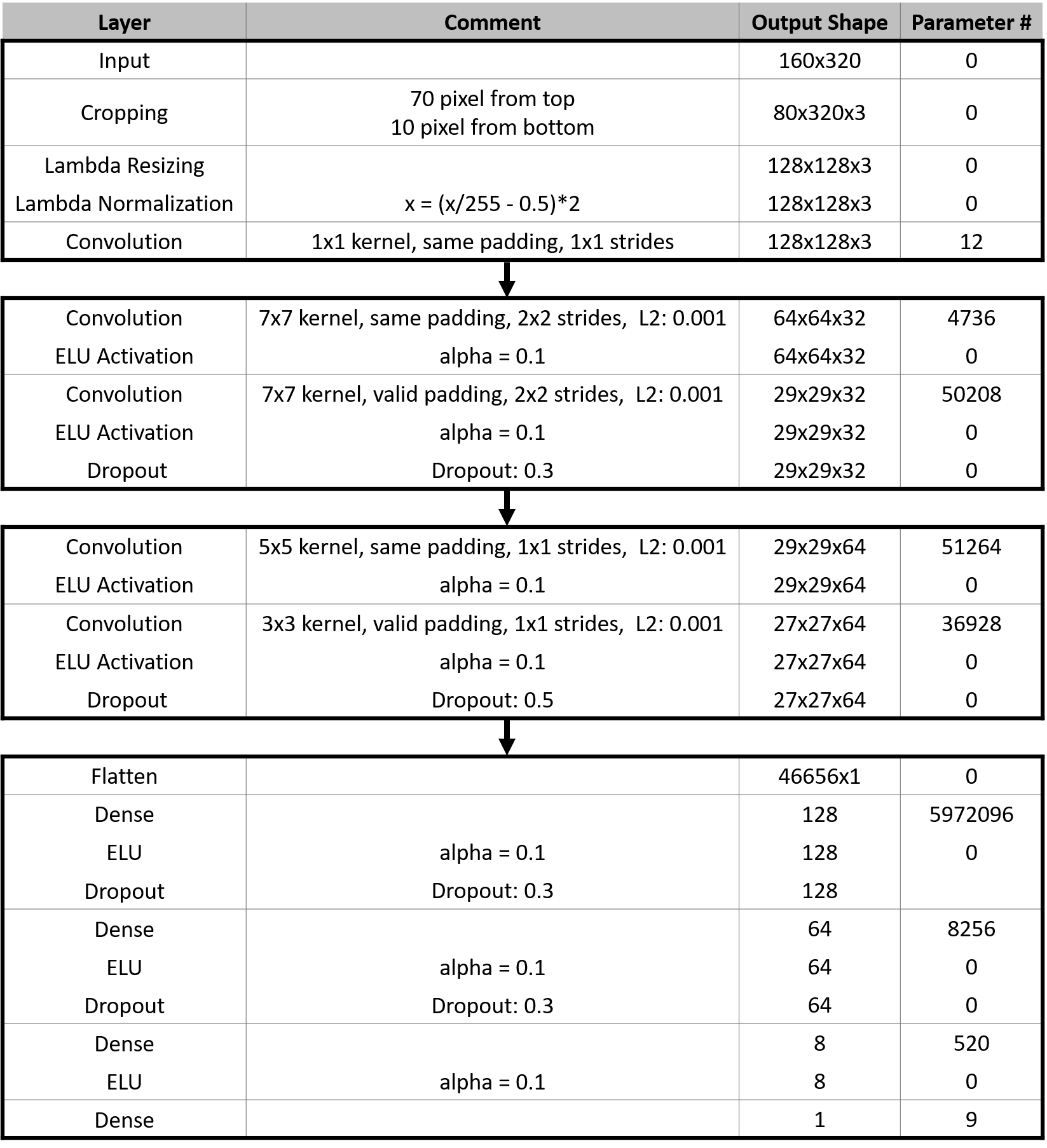
The model consists of a convolution neural network with different filter sizes and depths between 32 and 128 (architecture in model.py: lines 108 - 143). At first the input (images) get cropped by the keras Crop2D layer. 70 pixels from the top and 10 pixels from the bottom are cut from the image, because they contain no useful information for good driving.
Then there is a Lambda layer with uses a keras tensorflow backend function to resize the images to 128x128. The reason is a reduction in computational effort:
320 * (160-80) = 25600 px
128 * 128 = 16384 px
After this the images are normalized to -1;1 with the following equation:
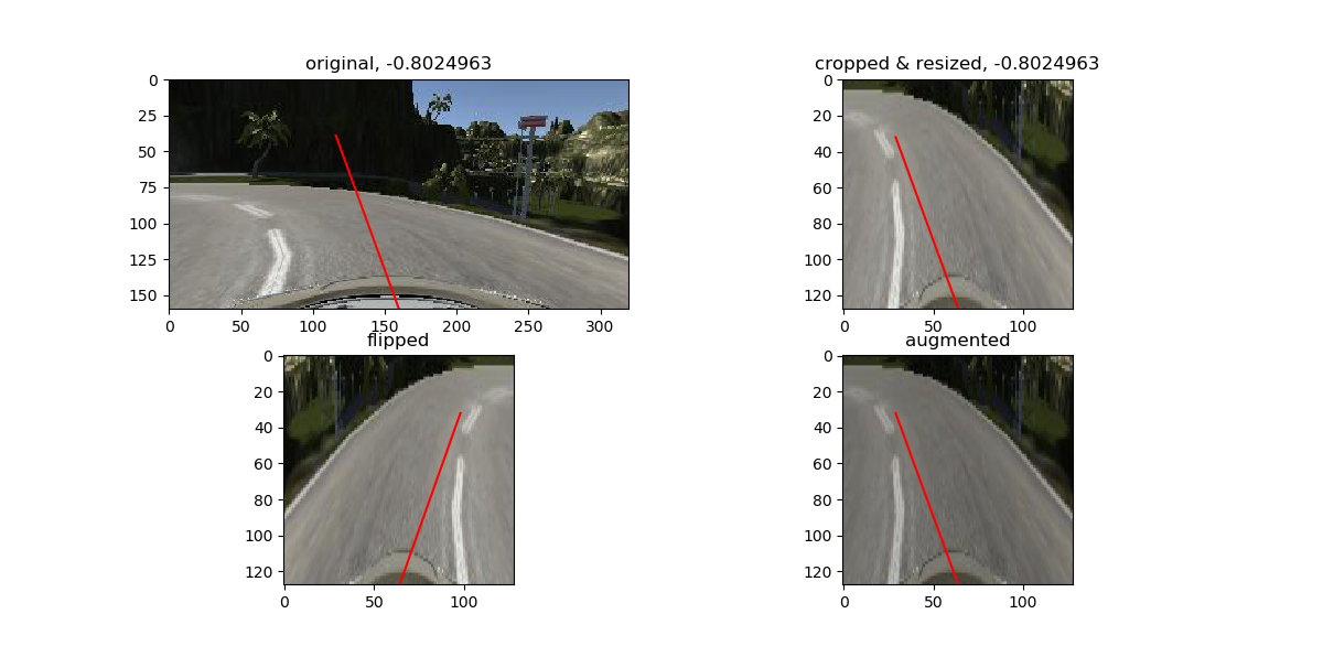
image_norm = (image/255 - 0.5) * 2This example shows the pipeline for image preprocessing, as well as a flipped and augmented example as mentioned above. The red line is a visualization of the steering angle:
Next layer is for figuring out the right colorspace, which proved its usefullness in the last project. The rest of the network is heavily inspired by Nvidia's network, but activations in the dense layers were swapped to ELUs.
MSE was choosen for representing the error.
Here is a visualization of the architecture:
-
The model contains dropout layers in order to reduce overfitting.
-
The model was trained and validated on different data sets to ensure that the model was not overfitting.
-
The model used the adam optimizer, which adapts the learning rate automatically to the training. It was set as 0.0001 at the beginning of training.
-
Desired batch size was chosen to 32 images, but the real batch size depends of the number of augmented images per image, if the flipped images are used, etc.. This will described in the next section 3.4.
-
Epoch size was set to 15, but a keras callback was implemented to save the model every epoch. Also an earlystopping callback was implemented, to end the training if the validation loss is greater than the epochs with a patience of 3 epoch.
-
The cleaned log data (size = 17433 samples) was split into training and validation data before feeding it to the batch generator in a ratio of 0.8 and 0.2, which gives them a size of 13946 and 3487 samples.
Due to restrictions in RAM(16GB) & VRAM(6GB) size of the used PC, a batch generator had to been implemented as soon as augmentation and using of left and right images started. This generator takes in the desired batch size, a sample list of logs and arguments which augmentation techniques to use.
Internally a generator batch size is calculated, the formula is:
gen_batch_size = batch_size // (2 * number of perspectives * (1+augmented_per_image))This gen_batch_size will always be smaller as the desired batch size. It is used for looping through the given log (training or validation) and generating batches for the fit_generator. Before feeding the batch generator and after batch generation before feeding to the fit_generator, a shuffling of the log data is done.
To define the "batches_in_epoch" in the fit_generator the real batch_size is:
real_batch_size = gen_batch_size * (2 * number of perspectives * (1+augmented_per_image))where as
batches_in_epoch = int(ceil(len(training_log / real_batch_size))This ensures that every sample with every choosen augmentation technique is used. For validation the "augmented_per_image" is set to zero.
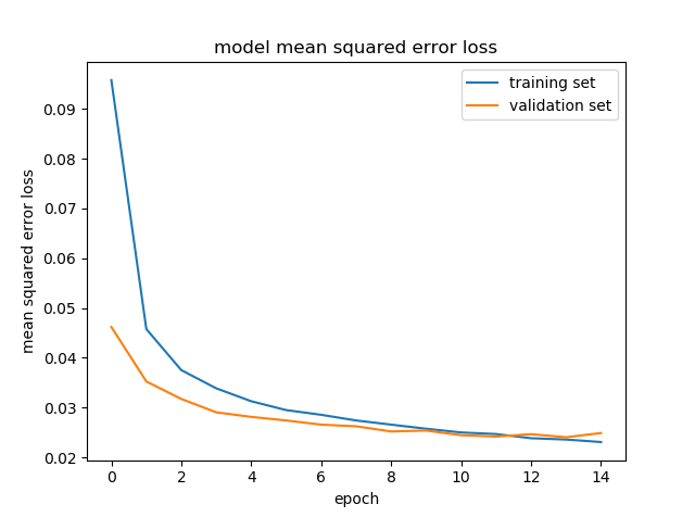
For the first training run the 13946 samples after cleaning and spliting were flipped, supplemented with the left & right images and augmented with 1 augmented image per sample. So all in all 167352 images for training. This diagram shows the progress of training & validation loss:
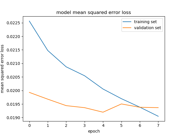
After this first training run, the models with the lowest validation losses were tested in the simulator. The one which seems to perform best was than again trained on all samples, but without left & right images and augmentation, only flipping.
The idea for this was: It's good to have a lot of sample to train the model to have basic understanding of how to drive. But the correction of the steering angle for left & right camera images will almost certainly introduce a small error, because this correction is just a guessed number, not proven right. For critical scenes like the sharp turns in track 2 even a small error can result in complete failure. So to train the model for good as possible steering "pure" data was used for the second training. This process significantly increased the performance in critical scenes.
The model was then again tested by running it through the simulator and ensuring that the vehicle could stay on the track. Here an interesting point was discovered: A small validation loss doesn't mean the model makes it succesfully trough both tracks, sometimes models with a higher validation loss performed better than the one with lower validation loss. An explanation for this could be: If all the validation loss is accumulated in then "extreme" scenes, where the steering angle is very high, the model performs weaker in the sharp turns in track 2 as a model with validation loss is distributed over all scenes. A investigation in this topic could be interesting.
At the end of the process, the vehicle is able to drive autonomously around the track without leaving the road.

