JutulDarcy.jl

Darcy-scale and subsurface flow (CO2 sequestration, gas/H2 storage, oil/gas fields) using Jutul.jl developed by the Computational Geosciences group at SINTEF Digital.

Key features

Written in pure Julia, with automatic differentiation and dynamic sparsity detection
Support for sensitivities with respect to any model parameters using the adjoint method
High performance assembly and linear solvers, with support for two-stage CPR BILU(0)-CPR Krylov solvers
Equation-of-state compositional, immiscible and black oil flow is supported and validated against existing simulators
Unstructured grids and complex cases input from the Matlab Reservoir Simulation Toolbox (MRST) using the jutul module.
Support for general multisegment wells with rigorous mass balance, complex well limits and time-dependent controls
3D visualization of grids and wells in JutulViz.jl
Interactive plotting of well curves

The compositional simulator has been matched against commercial offerings, AD-GPRS and MRST. The blackoil simulator has been validated on the standard SPE benchmarks (SPE1, SPE9, ...).

Example run times on benchmarks

Name	Cells	Report steps	Preconditioner	Time [s]
SPE1CASE2	300	120	block-ILU(0)	0.85
SPE9	9000	35	block-ILU(0)	9.30
Egg	18553	123	CPR-block-ILU(0)	22.5

Simulated with julia -O2, no threads.

A few of the packages used by Jutul and JutulDarcy

Jutul builds upon many of the excellent packages in the Julia ecosystem. Here are a few of them, and what they are used for:

ForwardDiff.jl implements the Dual number class used throughout the code
SparsityTracing.jl provides sparsity detection inside Jutul
Krylov.jl provides the iterative linear solvers
ILUZero.jl for ILU(0) preconditioners
AlgebraicMultigrid.jl for AMG preconditioners
Tullio.jl for automatically optimized loops and Polyester.jl for lightweight threads
TimerOutputs.jl and ProgressMeter.jl gives nice output to terminal
Makie.jl is used for the visualization features found in JutulViz.jl
MultiComponentFlash.jl provides many of the compositional features

...and many more, both directly in the Project.toml file and indirectly!

Getting started

Install Julia and add the package to your environment of choice (see details below).

Here is a self-contained example that demonstrates a conceptual multiphase flow simulation of CO2 injection with multisegment wells. To run the example, you need the following packages: Jutul for the grid structure, JutulDarcy for the reservoir simulator and Plots for the simple plotting used here. To add these, you can run the following in Julia:

using Pkg
Pkg.add("Jutul")
Pkg.add("JutulDarcy")
Pkg.add("Plots")

Once the packages are added and precompiled, you can run this example, for example by saving it in a file example.jl and running include("example.jl"). Note that the first time run will take some time due to compilation, but subsequent runs in the same session should be quick.

using Jutul, JutulDarcy, Plots
nx = ny = 10
nz = 2
day = 3600*24
bar = 1e5
g = CartesianMesh((nx, ny, nz), (2000.0, 1500.0, 50.0))
Darcy = 9.869232667160130e-13
K = repeat([0.1*Darcy], 1, number_of_cells(g))
res = discretized_domain_tpfv_flow(tpfv_geometry(g), porosity = 0.1, permeability = K)
# Vertical well in (1, 1, *), producer in (nx, ny, 1)
P = setup_vertical_well(g, K, 1, 1, name = :Producer)
I = setup_well(g, K, [(nx, ny, 1)], name = :Injector)
# Set up a two-phase immiscible system
phases = (AqueousPhase(), VaporPhase())
rhoWS = 1000.0; rhoGS = 700.0
rhoS = [rhoWS, rhoGS]
sys = ImmiscibleSystem(phases, reference_densities = rhoS)
model, parameters = setup_reservoir_model(res, sys, wells = [I, P])
# Replace the density function with our custom version for wells and reservoir
c = [1e-6/bar, 1e-5/bar]
ρ = ConstantCompressibilityDensities(p_ref = 1*bar, density_ref = rhoS, compressibility = c)
replace_variables!(model, PhaseMassDensities = ρ)
# Set up report time-steps, five years with 30 days each
dt = repeat([30.0]*day, 12*5)
# Inject two full pore-volumes (at reference conditions) of gas
rate_target = TotalRateTarget(2.0*sum(pore_volume(model))/sum(dt))
bhp_target = BottomHolePressureTarget(50*bar)
controls = Dict(:Injector => InjectorControl(rate_target, [0.0, 1.0], density = rhoGS),
                :Producer => ProducerControl(bhp_target))
# Wrap forces and initialize the state
forces = setup_reservoir_forces(model, control = controls)
state0 = setup_reservoir_state(model, Pressure = 150*bar, Saturations = [1.0, 0.0])
sim, config = setup_reservoir_simulator(model, state0, parameters)
states, reports = simulate!(sim, dt, forces = forces, config = config)
# Get output and plot results
wo = full_well_outputs(model, states, forces)
T = report_times(reports)./day
qgs = abs.(wo[:Producer][Symbol("Surface gas rate")])
qws = abs.(wo[:Producer][Symbol("Surface water rate")])
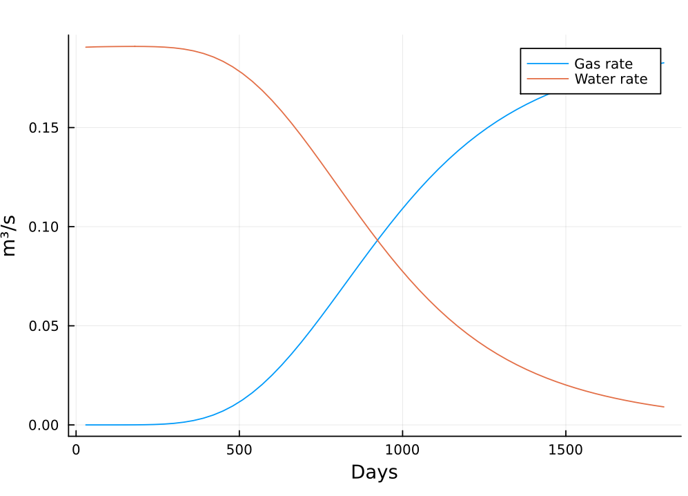
plt = plot(T, qgs, xlabel = "Days", ylabel="m³/s", label = "Gas rate")
plot!(T, qws, label = "Water rate")
display(plt)

We get a nice plot of the wells, and detailed statistics on the simulation time:

                    Number of iterations
╭────────────────────┬──────────┬──────────────┬──────────────┬────────┬───────╮
│ Type               │ Avg/step │ Avg/ministep │     Time per │ Wasted │ Total │
│                    │ 60 steps │ 64 ministeps │ Milliseconds │        │       │
├────────────────────┼──────────┼──────────────┼──────────────┼────────┼───────┤
│ Newtons            │      2.4 │         2.25 │       1.2936 │      0 │   144 │
│ Linearizations     │  3.46667 │         3.25 │       0.8956 │      0 │   208 │
│ Linear solver its. │     6.55 │      6.14062 │       0.4740 │      0 │   393 │
╰────────────────────┴──────────┴──────────────┴──────────────┴────────┴───────╯
                    Simulator timing
╭──────────────┬──────────────┬──────────┬──────────────╮
│ Name         │         Each │ Fraction │        Total │
│              │ Milliseconds │  Percent │ Milliseconds │
├──────────────┼──────────────┼──────────┼──────────────┤
│ Properties   │       0.2199 │  24.55 % │      45.7307 │
│ Assembly     │       0.1544 │  17.24 % │      32.1056 │
│ Linear solve │       0.3706 │  28.65 % │      53.3602 │
│ Update       │       0.0774 │   5.98 % │      11.1486 │
│ Convergence  │       0.1717 │  19.17 % │      35.7127 │
│ Input/Output │       0.0128 │   0.44 % │       0.8222 │
│ Other        │       0.0514 │   3.97 % │       7.3966 │
├──────────────┼──────────────┼──────────┼──────────────┤
│ Total        │       1.2936 │ 100.00 % │     186.2766 │
╰──────────────┴──────────────┴──────────┴──────────────╯

Additional examples and further reading

As per Julia tradition, the documentation is mostly missing at the moment. This can be considered an early beta release. Additional more complex examples are found in this repository.