This repository contains sample code to demonstrate Satellite Communications Forecasting use-cases. The associated blog is here.
It focuses on a Maritime shipping use-case, using Amazon Forecast to build a time series predictor model for each satellite beam in the ship(s) path, accounting for the impact of weather conditions in a given location. It then renders results in Amazon QuickSight BI tooling, displaying forecasted capacity needs, accuracy metrics, and which attributes most impact the model.

Multiple factors such as weather and the geographical location of the vessel in the beam impact data rates and therefore the usage of satellite capacity bandwidth.
Satellite Operators would like advance notice of capacity needs to plan out allocation, enabling the most efficient distribution of satellite capacity. This is where Amazon Forecast provides great benefit. Forecast can predict future capacity needs per beam leveraging historical bandwidth usage data and related time series such as weather metrics.
An accurate forecasting strategy can lead to lower costs (higher bandwidth utilization), and higher passenger satisfaction (e.g. successful capacity handling of demand surges).
The target time-series (TTS) data set required to predict future satellite capacity bandwidth needs is historical usage across each spot-beam over a period of time. Related datasets (RTS) are optional but serve to improve the model accuracy e.g. weather has a correlation with achievable data rates hence supplying weather data points, particularly severe weather, helps the Predictor.
We supply 14 days of historical and related time series data at 10-minute intervals. Why do we need so much? In general the model accuracy improves with more data however more specifically we want to identify any day of week or hour of day patterns such as the daily sea breeze effect in summer in Florida, US.
A lambda function is provided to generate the TTS and RTS datasets. Surge capacity windows and severe weather troughs are applied to subsets of the data to validate that Forecast can produce a model capable of handling typical SatCom scenarios such as congestion, "rain fade" etc
A Cloudformation template is supplied to deploy the lambda function automatically with the appropriate permissions. A pre-requisite is to supply the lambda as a zip file in an S3 bucket so that CloudFormation can reference it (the alternative is embedding the code in the YAML itself which can get a bit unwieldy!). Edit the path (folder) to the code zip in the CFN parameter settings as appropriate.
The results in csv, are posted to Amazon S3. It is suggested to create a folder structure similar to below. This enables Forecast Dataset import jobs to target the specific set of TTS or RTS files.
- satcom-forecast-bkt-12345/
- dataset/
- tts/
- rts/
- dataset/
An additional lambda function is provided to parse National Oceanic and Atmospheric Administration National Data Buoy Center historical and real-time datasets e.g. Station 41043
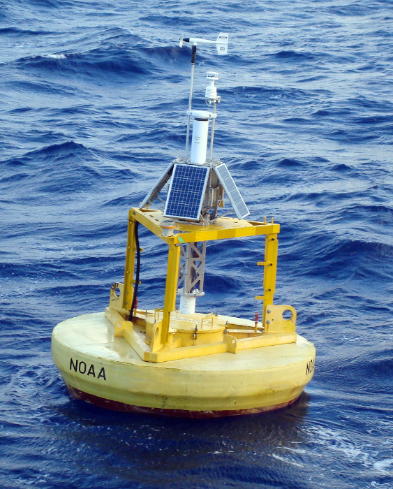
The key element is air-pressure (hPa) - a value below 990 indicates potentially severe weather. In the lambda, we peel out timestamp and air-pressure and then append day-of-week and hour-of-day to determine if there are any cyclical trends the model can identify.
Results are also posted to Amazon S3, under the rts/ folder.
A CloudFormation template is also supplied for this NOAA buoy parsing lambda function. A sample set of buoy data (station 41043) is supplied. You can get new datasets via wget at https://www.ndbc.noaa.gov/faq/rt_data_access.shtml The CFN parameters are similar to the previous lambda - however in this case we also add the buoy sample data file to the zipfile.
To improve the quality of the model there are several additional RTS datasets which could be injected such as: -
- more accurate weather forecast data using eg Accuweather APIs
- lost-lock activity e.g. if the communications link was broken at specific times in particular beams
- Carrier-to-Noise ratio (C/N), a measure of the received carrier strength relative to noise.
The entire set of operations can be done in the console, however a Jupyter notebook is provided to automate the sequence of following events: -

First up, is getting the correct permissions. An IAM role with full S3 access and Forecast access is required.
Next, historical bandwidth (TTS) and weather data (RTS) for 4 different spot-beams along the ship's route are imported to Amazon Forecast. Important variables to modify are the DATASET_FREQUENCY, schema(s), and the key (csv file or a folder/ in your S3 bucket). Since satellite bandwidth usage is dynamic, we set the DATASET_FREQUENCY to "10min". The schema, supplied in JSON, is different for TTS versus RTS: -
Historical bandwidth usage data
| Attribute | Type | Description |
|---|---|---|
| timestamp | timestamp | 10 min intervals in format yyyy-MM-dd HH:mm:ss |
| target_value | float | Satellite bandwidth usage historical data (MHz) |
| item_id | string | Spot-beam eg SpotH7, SpotH12 etc |
Weather historical and forecast data
| Attribute | Type | Description |
|---|---|---|
| timestamp | timestamp | 10 min intervals in format yyyy-MM-dd HH:mm:ss |
| air_pressure | integer | Barometric pressure of buoy in a given spot beam footprint |
| item_id | string | Spot-beam eg SpotH7, SpotH12 etc |
| day_of_week | string | Does day of week influence the model? |
| hour_of_day | string | Does hour of day influence the model? |
When the import(s) are complete, the notebook will return the job ARN with a status of ACTIVE.
The predictor step is then triggered. Be sure to set the FORECAST_HORIZON correctly. This is the number of time steps being forecasted. In our use-case the horizon is 144 ie 1 day (10 min granularity : 6 * 24)
We use an AutoPredictor model whereby each time series can receive a bespoke recipe – a blend of predictions underlying up to 6 different statistical and deep-learning models improving accuracy at every series. The net effect is higher accuracy, as outlined in the notebook section "Review accuracy metrics".
Our primary accuracy metric for this use-case is the P90 Weighted Quantile Loss (WQL), which indicates the confidence level of the true value being lower than the predicted value 90% of the time. This is important because Satellite Operators typically want to slightly overprovision ensuring consumers have enough bandwidth the majority of the time.
Finally, a forecast is generated with results exported to S3 for further ingestion by BI tools. A sample plot for SpotH12's next 24 hours capacity forecast at a P90 WQL is presented below: -

Simply change the ITEM_ID to query your target item of interest.
Additional metrics such as predictor explainability are also exported to S3 - this helps us refine the model by placing more emphasis on 1 RTS variable over another.
This completes the workflow.
To terminate all Forecast assets uncomment the "Clean-up" section
The same forecasting algorithms, ensembling techniques, explainability can now be done via SageMaker Autopilot timeseries.
The benefits of SageMaker Autopilot Timeseries over Amazon Forecast are: -
- accuracy metrics for all (6) algorithms leveraged in the AutoPredictor
- faster training time
- select which model to use (best candidate or otherwise)
- lower cost (particularly with Real Time Inference)
It is therefore recommended to use SageMaker Autopilot Timeseries over Amazon Forecast for new prediction use-cases.
A Jupyter notebook demonstrating how to perform satellite capacity forecasting with SageMaker Autopilot is here along with a complete README
See CONTRIBUTING for more information.
This library is licensed under the MIT-0 License. See the LICENSE file.