Clustering

A demo on identifying clusters in a data set using the D-Wave quantum computer.

When dealing with large data sets, we do not always have neatly labeled data (i.e. most, if not all, the data could be unlabeled). However, all is not lost as we can still extract insights from this data through clustering.

For example, when dealing with housing data---namely, square footage and price---we can identify clusters in that data which may be indicative of different neighborhoods. Another example could be having a boolean vector of TV shows that consumers watch; clusters in this data could help identify a particular consumer demographic.

As well, if we do have a few labelled data points in our data set, we could potentially label the entire cluster based on these.

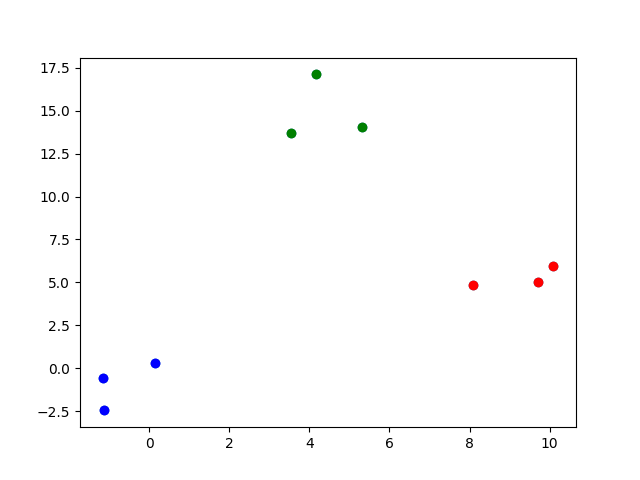
Figure: A data set of nine points that have been divided into three clusters (shown with different colors).

Usage

To run the demo with a simple, hardcoded data set:

python clustering.py

To run the same demo with a slightly more sophisticated data set:

python example_clusters.py

This provides a visualization of the problem on the D-Wave problem inspector, and plots of the original data set and its solution.

Code Overview

The D-Wave quantum computer accepts problems formulated mathematically in Binary Quadratic Model (BQM) format. The goal here is to build a BQM such that it represents our clustering problem. Namely, we want a BQM such that a low-energy solution found by the D-Wave quantum computer would correspond to a solution to our clustering problem.

Key properties of the clustering problem that we need to capture in our BQM:

Each data point can only be a part of one cluster
Data points that are close together should be a part of the same cluster
Data points that are far apart should be in different clusters

Code Specifics

Let's go through how we implement each of the key properties of our clustering problem.

Each data point can only join one cluster

The code is only considering three different cluster labels: red, green, and blue.
Since a qubit can only end up in one of two states (i.e. it can only answer yes or no questions), each data point has three nodes associated to it: <coordinate>.r, <coordinate>.g, and <coordinate>.b. That way, we can answer yes-no questions for whether a specific coordinate is in a particular colour cluster.
The rule that a data point may only join one cluster is represented by the variable choose_one_group (shown below). Each three-item-tuple below can be interpreted as (<join-red>, <join-green>, <join-blue>), where the 1s and 0s indicate true and false, respectively. Hence, the choose_one_group is a set of all valid states. (e.g. (1, 1, 0) is not valid because a data point is not allowed to be in both red and green clusters at once).
```
choose_one_group = {(0, 0, 1), (0, 1, 0), (1, 0, 0)}
```
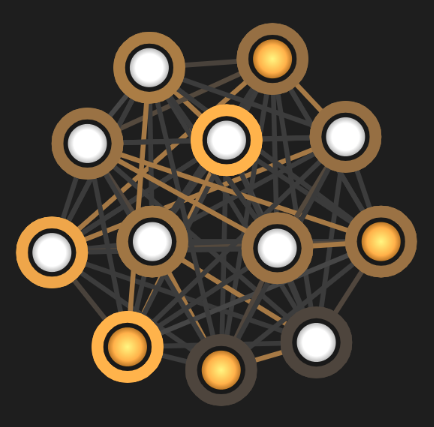
You can easily see this "choose one group" constraint in the D-Wave inspector. The image below has four data points (as seen in clustering.py). Each of the four data points has three nodes associated with it - <coordinate>.r, <coordinate.g>, and <coordinate.b> - hence the twelve nodes below.
A particular data point's set of three nodes can actually be identified in the graph below. By noting the yellow triangles below, we can see that one vertex is selected (in yellow) and two vertices are not selected (in white).

In the actual D-Wave Inspector, you can hover over these nodes and find out which data point and colour they represent and the BQM weights that are placed on them.

Close data points should be in the same cluster

If we set BQM weights such that clustering close data points has lower-energy solutions, when the quantum computer minimizes the BQM, it finds good solutions to the clustering problem.
These weights are dependent on distance. In order to keep the weights within a reasonable range, the distances are all scaled with respect to the max_distance, the largest distance between any two points in the data set.
Below is the function used to determine the weight to encourage close together points to be in the same cluster
```
d = get_distance(coord0, coord1) / max_distance  # rescale distance
weight = -math.cos(d*math.pi)
```
We can apply many different types of functions for generating the weight. In this case, we chose a cosine function. The main idea is that we simply need short distances (nearby points) to generate a strong negative value that contributes to clustering these points, while points with large distances are only mildly affected.

Far-apart data points should be in different clusters

Here, we want to encourage far apart data points to be in different clusters. Again, since the D-Wave quantum computer seeks low-energy configurations, we need to make far apart data points correspond to lower energy.
We do this by choosing a strong negative weight for far apart points. Hence, the choice of the tanh function.
```
d = math.sqrt(get_distance(coord0, coord1) / max_distance)
weight = -math.tanh(d) * 0.1
```
Note that a scalar of 0.1 was applied in order to prevent this weight from overwhelming the other weights in the BQM. The 0.1 is arbitrary and was found by tinkering with the code.

License

Released under the Apache License 2.0. See LICENSE file.

ayazskhan/clustering