kernelgon

The function kernelgon will calculate and plot polygons in base R graphics based on a collection of points stored as an $n$ by 2 matrix.

Requirements:

R (v 3.3.2 or greater) https://cran.r-project.org/
ks package (v 1.11.2 or greater)
concaveman package (v 1.0.0 or greater)
igraph package (v 1.2.1 or greater)

Installation notes

Some of the above libraries may require you first install other programs outside of R. On Ubuntu 17.04, you may need to install libudunits2.so first via

sudo apt-get install libudunits2-dev

in the terminal. A concaveman dependency, the V8 package, may also need a the libv8 library file using

sudo apt-get install -y libv8-3.14-dev

Usage

The package and function kernelgon simply combines the kernel density estimation of the ks package with the polygon-tracing abilities of concaveman. We can set plot the intervals on any $n$ by 2 matrix of coordinates via


d <- data.frame(x = rnorm(500, 0, 1), y = rnorm(500, 100, 5))

plot(d)
kernelgon(d, lty = 2)

For important theoretical reasons, the default highest-density interval is 89%, implying about that many observations should fall within this area. This can be changed to any probability interval by the prob argument. Because kernelgon works exactly like polygon, it accepts any of the normal arguments and is extremely flexible.

plot(d)
kernelgon(d, prob = 0.5, lty = 2, border = "blue", lwd = 2)
kernelgon(d, prob = 0.95, lty = 3, border = "red", lwd = 2)

The res argument controls the line resolution; too small and the lines look jagged, but too large and the polygon loses detail.

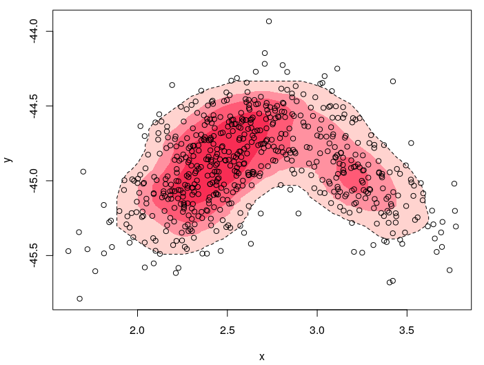
The kernelgon function can handle unusually-shaped, multi-peak probability landscapes. Here is an example:


correlator <- function(r, x.mean=0, x.sd=1, y.mean=0, y.sd=1, n=1000){
    x <- rnorm(n, mean=x.mean, sd=x.sd)
    y <- rnorm(n, mean=r*(y.sd/x.sd)*(x-x.mean)+y.mean, sd=sqrt((1-r^2))*y.sd)
    data.frame(x,y)
}

col_alpha <- function (acol, alpha = 0.2){
    acol <- col2rgb(acol)
    acol.red <- acol["red",]/255
    acol.green <- acol["green",]/255
    acol.blue <- acol["blue",]/255
    acol <- mapply(function(red, green, blue, alphas) rgb(red, green, blue, alphas), acol.red, acol.green, acol.blue, alpha)
    return(as.character(acol))
}

rose <- c(
  "#FFA8A0", 
  #"#FF7489", 
  "#FF5072", 
  "#FF254D", 
  "#F10033",
  "white"
)

n_obs <- 400

base <- correlator(0.6, x.mean = 2.4, x.sd = 0.25, y.mean = -44.9, y.sd = 0.3, n = 400)
add <- correlator(-0.6, x.mean = 3.2, x.sd = 0.25, y.mean = -44.9, y.sd = 0.3, n = 200)
d <- rbind(base, add)

plot(d, col = NULL)
kernelgon(d, prob = 0.89, col = col_alpha(rose[1], 0.5), lty = 2)
kernelgon(d, prob = 0.7, col = col_alpha(rose[2], 0.5), border = NA)
kernelgon(d, prob = 0.5, col = col_alpha(rose[3], 0.5), border = NA)
kernelgon(d, prob = 0.25, col = col_alpha(rose[4], 0.5), border = NA)
points(d)

babeheim/kernelgon

kernelgon

Installation notes

Usage