I have implemented Monte Carlo model in MATLAB.
Algorithm:
- First pick a location at random and then a neighbor of that location at random. Consider the change of state from its current one to a random new state according to the following scheme:
- For each of the z neighbors and N total locations, evaluate the following Hamiltonian:
$$H = \frac{J}{2}\sum_{i=1}^{N}\sum_{j=1}^{z}[1 - \delta(S_i,S_j)]$$ Here, J is the strength of the grain boundary energy, S is the state at that position and$\delta$ is the Kronecker delta.- Evaluate the probability
$p = exp\Big[ \frac{-\Delta H}{k_BT} \Big]$ for the difference of Hamiltonian before and after flip of state. Choose a higher T if faster changes are desired in the microstructure.- Generate a random number z between 0 and 1. Decide on whether to accept the flip if
$z\leq p$ and to reject the flip if$z>p$ - Store the new state and proceed to next location.
- Once all the locations are visited, store the map of states and proceed to next time step.
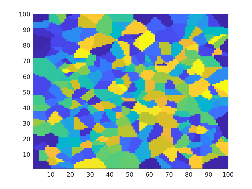
For getting a microstructure I used Delaunay triangulation using a function in MATLAB and discretized it to run the algorithm on it. We get a figure as shown below:

This code was developed as a part of the course Computational Materials Engineering Lab During the simulations, images are stored in the folder images_output Few example images of simulations are provide in Example images folder for reference