Welcome to the estimation project. In this project, you will be developing the estimation portion of the controller used in the CPP simulator. By the end of the project, your simulated quad will be flying with your estimator and your custom controller (from the previous project)!
This README is broken down into the following sections:
- Setup - the environment and code setup required to get started and a brief overview of the project structure
- The Tasks - the tasks you will need to complete for the project
- Tips and Tricks - some additional tips and tricks you may find useful along the way
- Submission - overview of the requirements for your project submission
This project will continue to use the C++ development environment you set up in the Controls C++ project.
- Clone the repository
git clone https://github.com/udacity/FCND-Estimation-CPP.git
-
Import the code into your IDE like done in the Controls C++ project
-
You should now be able to compile and run the estimation simulator just as you did in the controls project
For this project, you will be interacting with a few more files than before.
-
The EKF is already partially implemented for you in
QuadEstimatorEKF.cpp -
Parameters for tuning the EKF are in the parameter file
QuadEstimatorEKF.txt -
When you turn on various sensors (the scenarios configure them, e.g.
Quad.Sensors += SimIMU, SimMag, SimGPS), additional sensor plots will become available to see what the simulated sensors measure. -
The EKF implementation exposes both the estimated state and a number of additional variables. In particular:
-
Quad.Est.E.Xis the error in estimated X position from true value. More generally, the variables in<vehicle>.Est.E.*are relative errors, though some are combined errors (e.g. MaxEuler). -
Quad.Est.S.Xis the estimated standard deviation of the X state (that is, the square root of the appropriate diagonal variable in the covariance matrix). More generally, the variables in<vehicle>.Est.S.*are standard deviations calculated from the estimator state covariance matrix. -
Quad.Est.Dcontains miscellaneous additional debug variables useful in diagnosing the filter. You may or might not find these useful but they were helpful to us in verifying the filter and may give you some ideas if you hit a block.
-
In the config directory, in addition to finding the configuration files for your controller and your estimator, you will also see configuration files for each of the simulations. For this project, you will be working with simulations 06 through 11 and you may find it insightful to take a look at the configuration for the simulation.
As an example, if we look through the configuration file for scenario 07, we see the following parameters controlling the sensor:
# Sensors
Quad.Sensors = SimIMU
# use a perfect IMU
SimIMU.AccelStd = 0,0,0
SimIMU.GyroStd = 0,0,0
This configuration tells us that the simulator is only using an IMU and the sensor data will have no noise. You will notice that for each simulator these parameters will change slightly as additional sensors are being used and the noise behavior of the sensors change.
Once again, you will be building up your estimator in pieces. At each step, there will be a set of success criteria that will be displayed both in the plots and in the terminal output to help you along the way.
Project outline:
- Step 1: Sensor Noise
- Step 2: Attitude Estimation
- Step 3: Prediction Step
- Step 4: Magnetometer Update
- Step 5: Closed Loop + GPS Update
- Step 6: Adding Your Controller
For the controls project, the simulator was working with a perfect set of sensors, meaning none of the sensors had any noise. The first step to adding additional realism to the problem, and developing an estimator, is adding noise to the quad's sensors. For the first step, you will collect some simulated noisy sensor data and estimate the standard deviation of the quad's sensor.
-
Run the simulator in the same way as you have before
-
Choose scenario
06_NoisySensors. In this simulation, the interest is to record some sensor data on a static quad, so you will not see the quad move. You will see two plots at the bottom, one for GPS X position and one for The accelerometer's x measurement. The dashed lines are a visualization of a single standard deviation from 0 for each signal. The standard deviations are initially set to arbitrary values (after processing the data in the next step, you will be adjusting these values). If they were set correctly, we should see ~68% of the measurement points fall into the +/- 1 sigma bound. When you run this scenario, the graphs you see will be recorded to the following csv files with headers:config/log/Graph1.txt(GPS X data) andconfig/log/Graph2.txt(Accelerometer X data). -
Process the logged files to figure out the standard deviation of the the GPS X signal and the IMU Accelerometer X signal.
-
Plug in your result into the top of
config/6_Sensornoise.txt. Specially, set the values forMeasuredStdDev_GPSPosXYandMeasuredStdDev_AccelXYto be the values you have calculated. -
Run the simulator. If your values are correct, the dashed lines in the simulation will eventually turn green, indicating you’re capturing approx 68% of the respective measurements (which is what we expect within +/- 1 sigma bound for a Gaussian noise model)
Success criteria: Your standard deviations should accurately capture the value of approximately 68% of the respective measurements.
NOTE: Your answer should match the settings in SimulatedSensors.txt, where you can also grab the simulated noise parameters for all the other sensors.
Now let's look at the first step to our state estimation: including information from our IMU. In this step, you will be improving the complementary filter-type attitude filter with a better rate gyro attitude integration scheme.
-
Run scenario
07_AttitudeEstimation. For this simulation, the only sensor used is the IMU and noise levels are set to 0 (seeconfig/07_AttitudeEstimation.txtfor all the settings for this simulation). There are two plots visible in this simulation.- The top graph is showing errors in each of the estimated Euler angles.
- The bottom shows the true Euler angles and the estimates. Observe that there’s quite a bit of error in attitude estimation.
-
In
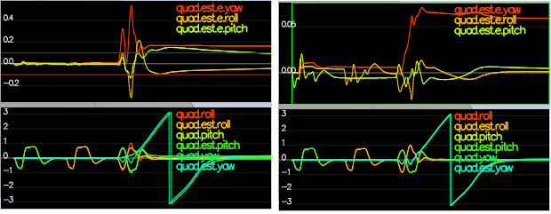
QuadEstimatorEKF.cpp, you will see the functionUpdateFromIMU()contains a complementary filter-type attitude filter. To reduce the errors in the estimated attitude (Euler Angles), implement a better rate gyro attitude integration scheme. You should be able to reduce the attitude errors to get within 0.1 rad for each of the Euler angles, as shown in the screenshot below.
In the screenshot above the attitude estimation using linear scheme (left) and using the improved nonlinear scheme (right). Note that Y axis on error is much greater on left.
Success criteria: Your attitude estimator needs to get within 0.1 rad for each of the Euler angles for at least 3 seconds.
Hint: see section 7.1.2 of Estimation for Quadrotors for a refresher on a good non-linear complimentary filter for attitude using quaternions.
In this next step you will be implementing the prediction step of your filter.
-
Run scenario
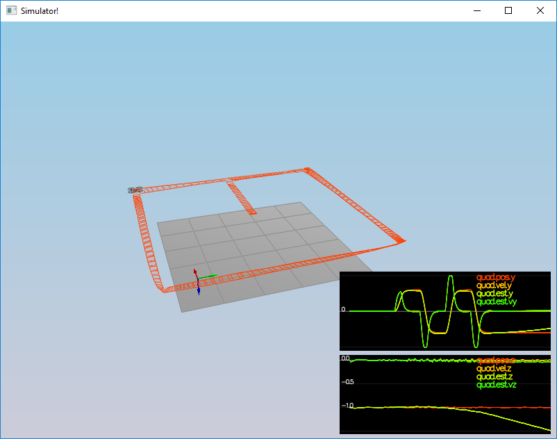
08_PredictState. This scenario is configured to use a perfect IMU (only an IMU). Due to the sensitivity of double-integration to attitude errors, we've made the accelerometer update very insignificant (QuadEstimatorEKF.attitudeTau = 100). The plots on this simulation show element of your estimated state and that of the true state. At the moment you should see that your estimated state does not follow the true state. -
In
QuadEstimatorEKF.cpp, implement the state prediction step in thePredictState()functon. If you do it correctly, when you run scenario08_PredictStateyou should see the estimator state track the actual state, with only reasonably slow drift, as shown in the figure below:
-
Now let's introduce a realistic IMU, one with noise. Run scenario
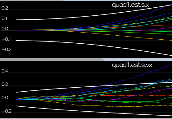
09_PredictionCov. You will see a small fleet of quadcopter all using your prediction code to integrate forward. You will see two plots:- The top graph shows 10 (prediction-only) position X estimates
- The bottom graph shows 10 (prediction-only) velocity estimates You will notice however that the estimated covariance (white bounds) currently do not capture the growing errors.
-
In
QuadEstimatorEKF.cpp, calculate the partial derivative of the body-to-global rotation matrix in the functionGetRbgPrime(). Once you have that function implement, implement the rest of the prediction step (predict the state covariance forward) inPredict().
Hint: see section 7.2 of Estimation for Quadrotors for a refresher on the the transition model and the partial derivatives you may need
Hint: When it comes to writing the function for GetRbgPrime, make sure to triple check you've set all the correct parts of the matrix.
Hint: recall that the control input is the acceleration!
- Run your covariance prediction and tune the
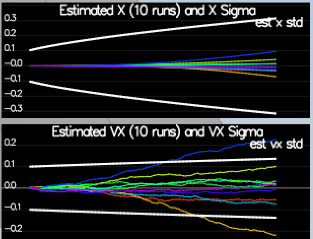
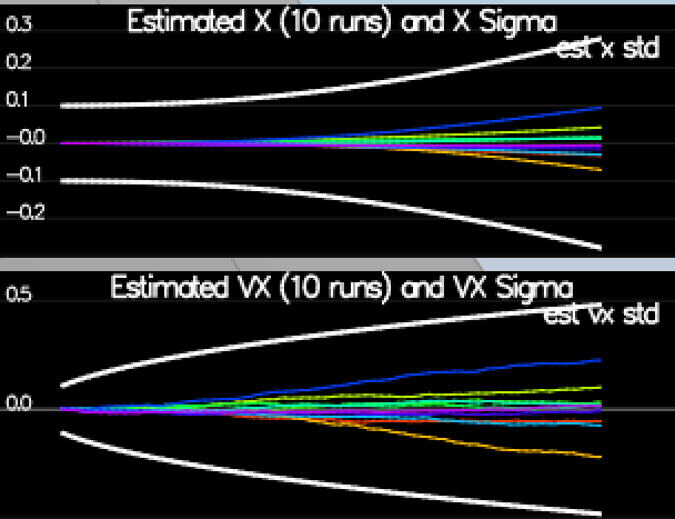
QPosXYStdand theQVelXYStdprocess parameters inQuadEstimatorEKF.txtto try to capture the magnitude of the error you see. Note that as error grows our simplified model will not capture the real error dynamics (for example, specifically, coming from attitude errors), therefore try to make it look reasonable only for a relatively short prediction period (the scenario is set for one second). A good solution looks as follows:
Looking at this result, you can see that in the first part of the plot, our covariance (the white line) grows very much like the data.
If we look at an example with a QPosXYStd that is much too high (shown below), we can see that the covariance no longer grows in the same way as the data.
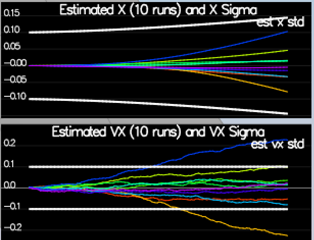
Another set of bad examples is shown below for having a QVelXYStd too large (first) and too small (second). As you can see, once again, our covariances in these cases no longer model the data well.
Success criteria: This step doesn't have any specific measurable criteria being checked.
Up until now we've only used the accelerometer and gyro for our state estimation. In this step, you will be adding the information from the magnetometer to improve your filter's performance in estimating the vehicle's heading.
-
Run scenario
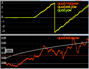
10_MagUpdate. This scenario uses a realistic IMU, but the magnetometer update hasn’t been implemented yet. As a result, you will notice that the estimate yaw is drifting away from the real value (and the estimated standard deviation is also increasing). Note that in this case the plot is showing you the estimated yaw error (quad.est.e.yaw), which is drifting away from zero as the simulation runs. You should also see the estimated standard deviation of that state (white boundary) is also increasing. -
Tune the parameter
QYawStd(QuadEstimatorEKF.txt) for the QuadEstimatorEKF so that it approximately captures the magnitude of the drift, as demonstrated here:
- Implement magnetometer update in the function
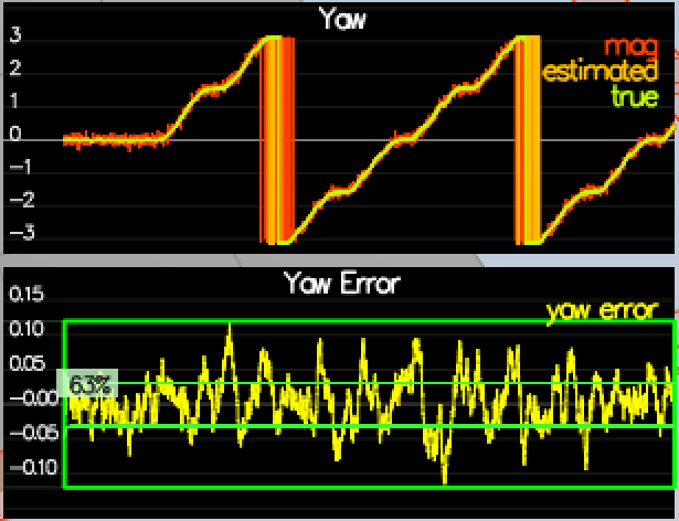
UpdateFromMag(). Once completed, you should see a resulting plot similar to this one:
Success criteria: Your goal is to both have an estimated standard deviation that accurately captures the error and maintain an error of less than 0.1rad in heading for at least 10 seconds of the simulation.
Hint: after implementing the magnetometer update, you may have to once again tune the parameter QYawStd to better balance between the long term drift and short-time noise from the magnetometer.
Hint: see section 7.3.2 of Estimation for Quadrotors for a refresher on the magnetometer update.
-
Run scenario
11_GPSUpdate. At the moment this scenario is using both an ideal estimator and and ideal IMU. Even with these ideal elements, watch the position and velocity errors (bottom right). As you see they are drifting away, since GPS update is not yet implemented. -
Let's change to using your estimator by setting
Quad.UseIdealEstimatorto 0 inconfig/11_GPSUpdate.txt. Rerun the scenario to get an idea of how well your estimator work with an ideal IMU. -
Now repeat with realistic IMU by commenting out these lines in
config/11_GPSUpdate.txt:
#SimIMU.AccelStd = 0,0,0
#SimIMU.GyroStd = 0,0,0
-
Tune the process noise model in
QuadEstimatorEKF.txtto try to approximately capture the error you see with the estimated uncertainty (standard deviation) of the filter. -
Implement the EKF GPS Update in the function
UpdateFromGPS(). -
Now once again re-run the simulation. Your objective is to complete the entire simulation cycle with estimated position error of < 1m (you’ll see a green box over the bottom graph if you succeed). You may want to try experimenting with the GPS update parameters to try and get better performance.
Success criteria: Your objective is to complete the entire simulation cycle with estimated position error of < 1m.
Hint: see section 7.3.1 of Estimation for Quadrotors for a refresher on the GPS update.
At this point, congratulations on having a working estimator!
Up to this point, we have been working with a controller that has been relaxed to work with an estimated state instead of a real state. So now, you will see how well your controller performs and de-tune your controller accordingly.
-
Replace
QuadController.cppwith the controller you wrote in the last project. -
Replace
QuadControlParams.txtwith the control parameters you came up with in the last project. -
Run scenario
11_GPSUpdate. If your controller crashes immediately do not panic. Flying from an estimated state (even with ideal sensors) is very different from flying with ideal pose. You may need to de-tune your controller. Decrease the position and velocity gains (we’ve seen about 30% detuning being effective) to stabilize it. Your goal is to once again complete the entire simulation cycle with an estimated position error of < 1m.
Hint: you may find it easiest to do your de-tuning as a 2 step process by reverting to ideal sensors and de-tuning under those conditions first.
Success criteria: Your objective is to complete the entire simulation cycle with estimated position error of < 1m.
-
When it comes to transposing matrices,
.transposeInPlace()is the function you want to use to transpose a matrix -
The Estimation for Quadrotors document contains a helpful mathematical breakdown of the core elements on your estimator
For this project, you will need to submit:
-
a completed estimator that meets the performance criteria for each of the steps by submitting:
QuadEstimatorEKF.cppconfig/QuadEstimatorEKF.txt
-
a re-tuned controller that, in conjunction with your tuned estimator, is capable of meeting the criteria laid out in Step 6 by submitting:
QuadController.cppconfig/QuadControlParams.txt
-
a write up addressing all the points of the rubric
Thanks to Fotokite for the initial development of the project code and simulator.
