Deep learning is an efficient technique to solve complex problems, and the “science” part of data science is all about experimenting with different settings and comparing results. Using Watson Studio, you can easily architect a neural network using a friendly GUI. In this tutorial, we will build a model that detects signature fraud by building a deep neural network. You will learn how to use Watson Studio’s Neural Network Modeler to quickly prototype a neural network architecture and test it, before calling its API and letting it score an image remotely. The dataset contains images of signatures, some genuine and some were simulated (fraud). The original source of the dataset is the ICFHR 2010 Signature Verification Competition. Images are resized to 32×32 pixels and are stored as numpy arrays in a pickled format.
If you have completed the preparation guide, you should have done the following:
- Created an IBM Cloud account
- Provisioned an Object Storage instance
- Provisioned a Machine Learning service instance
- Provisioned a Watson Studio service instance
- Installed the Watson Machine Learning Python SDK
If you have not, follow this link and complete the steps therein before continuing with the workshop.
Before we start building our neural network, we will need to upload files containing training, validation, and test data to our Cloud Object Storage instance. First, you need to download the assets.zip folder from this repository to somewhere you can find it easily. Next, unzip the assets folder, and make sure you can locate three different data files: training_data.pickle, validation_data.pickle and test_data.pickle. The .zip-file also contains two other files; evaluation_data.pickle and evaluate.py. These two are used in the final step of this workshop where we want to score an image by calling the API of a model we have deployed.
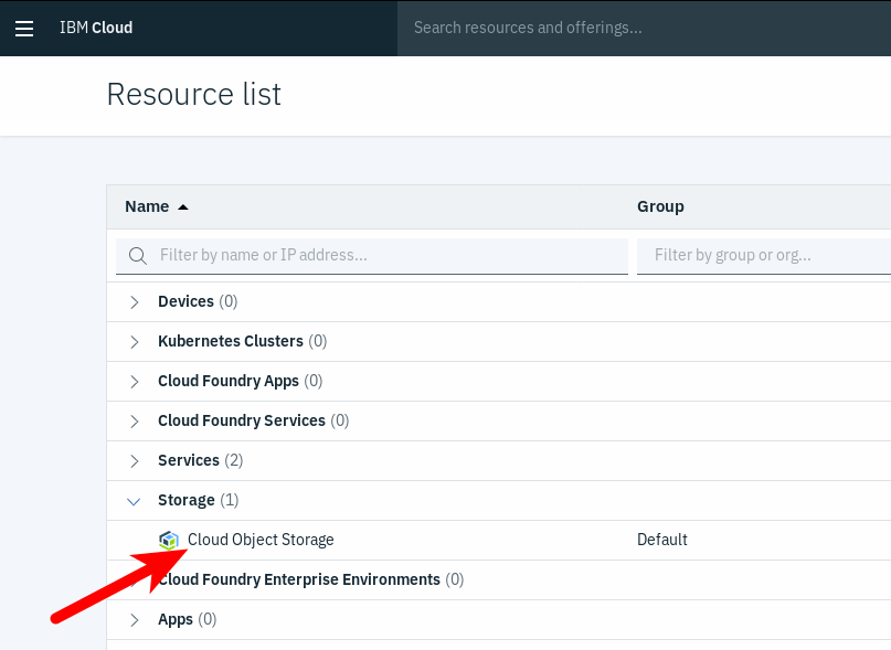
Go to your dashboard on IBM Cloud and click on Storage under the Resource summary. Then click on your Cloud Object Storage instance:
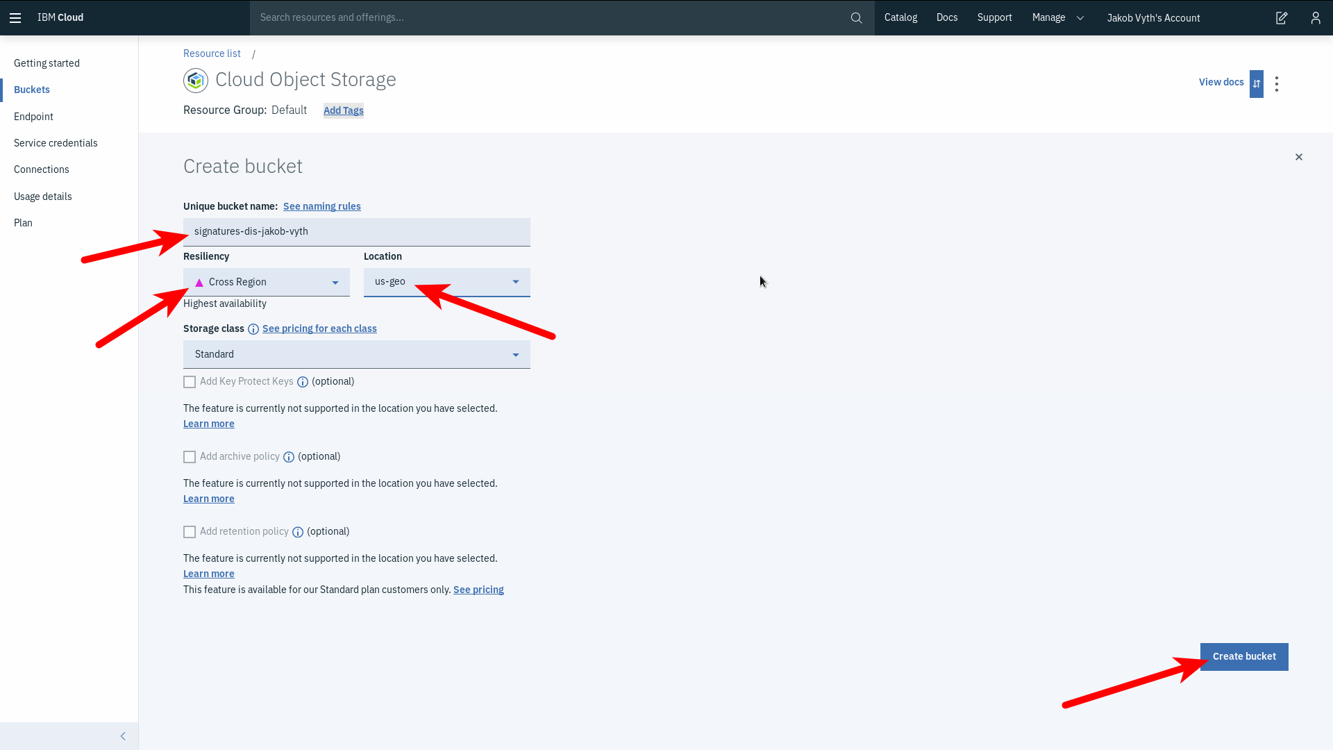
Create a bucket to store the data in by selecting Create bucket. Storing the data in a bucket makes it easier to locate when working with Watson Studio’s Neural Network Modeler. You can name the bucket anything, but it must be globally unique to IBM Cloud Object Storage. Make sure that resiliency is set to Cross Region and location to us-geo before clicking Create bucket:
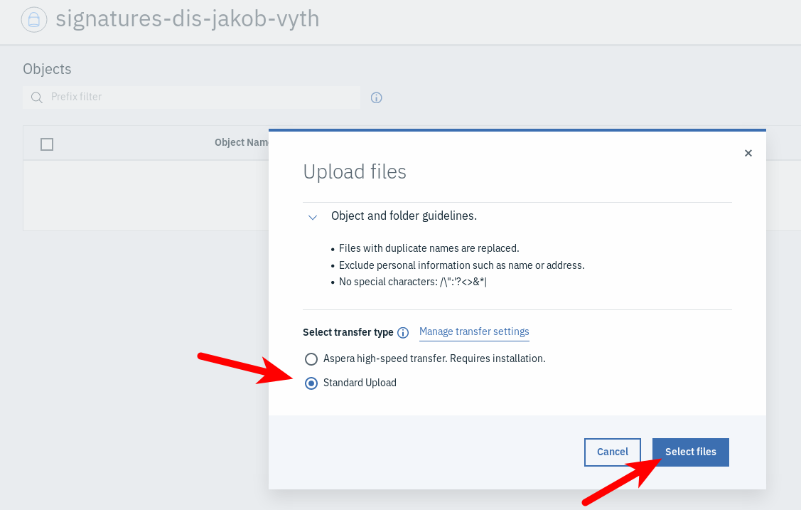
Start adding files to your newly created bucket by clicking the Upload button on the top right corner of the page and selecting the Files option from the drop-down menu. Select Standard Upload and click Select files:
Choose the three files named training_data.pickle, validation_data.pickle and test_data.pickle from where you unzipped the assets folder before. You should be prompted to confirm the file selections. Click Upload to proceed. Now you should see the page displaying the files you just uploaded:
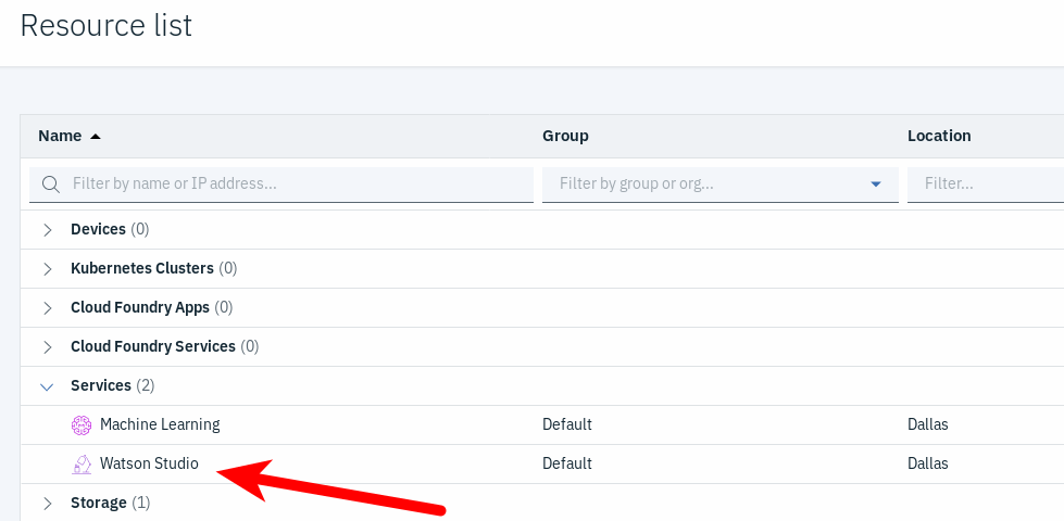
Go back to the dashboard and click on Services under the Resource summary. Then click on your Watson Studio instance:
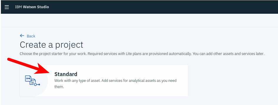
Next, click Get Started and then Create a project. Choose the Standard option:
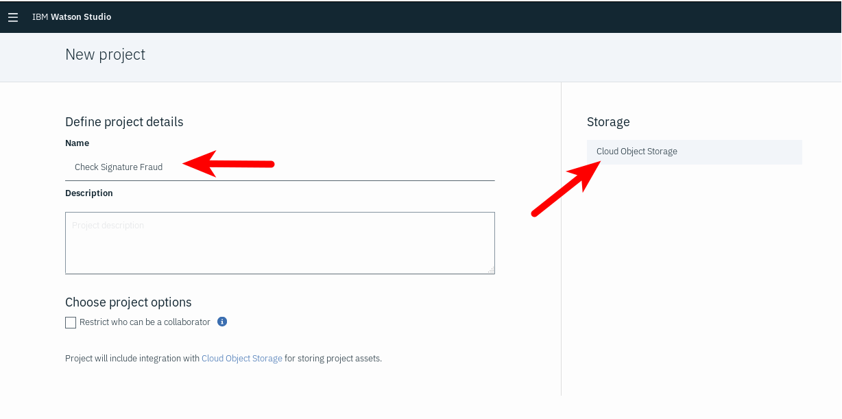
Give your project a name and make sure that your Cloud Object Storage instance shows up under Storage on the right side of the screen:
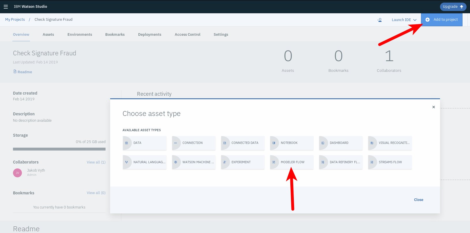
Click Create in the bottom right. You are now ready to work with Watson Studio! Create a Modeler Flow by clicking Add to project and then selecting Modeler Flow:
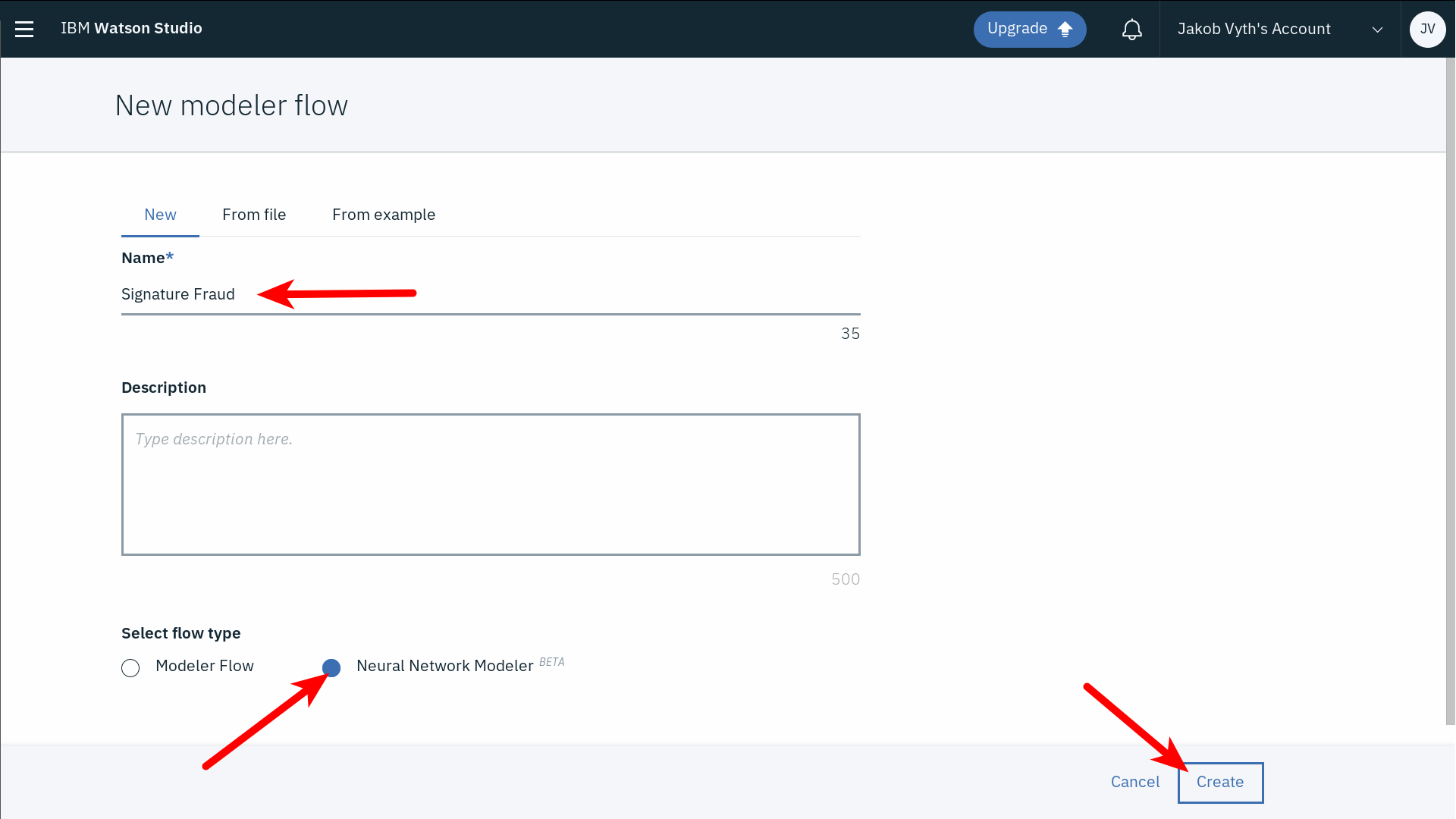
Give your model a name, select Neural Network Modeler, and click Create:
Once the previous step is successful, you will be presented with the Modeler Canvas. This is where you will build your Neural Network which will be represented in a graphical form instead of code. You will find a sidebar on the left of the screen containing all available neural network component, named Palette:
The whole idea here is to drag and drop nodes representing the different layers of a Neural Network and connecting them to create a Flow.
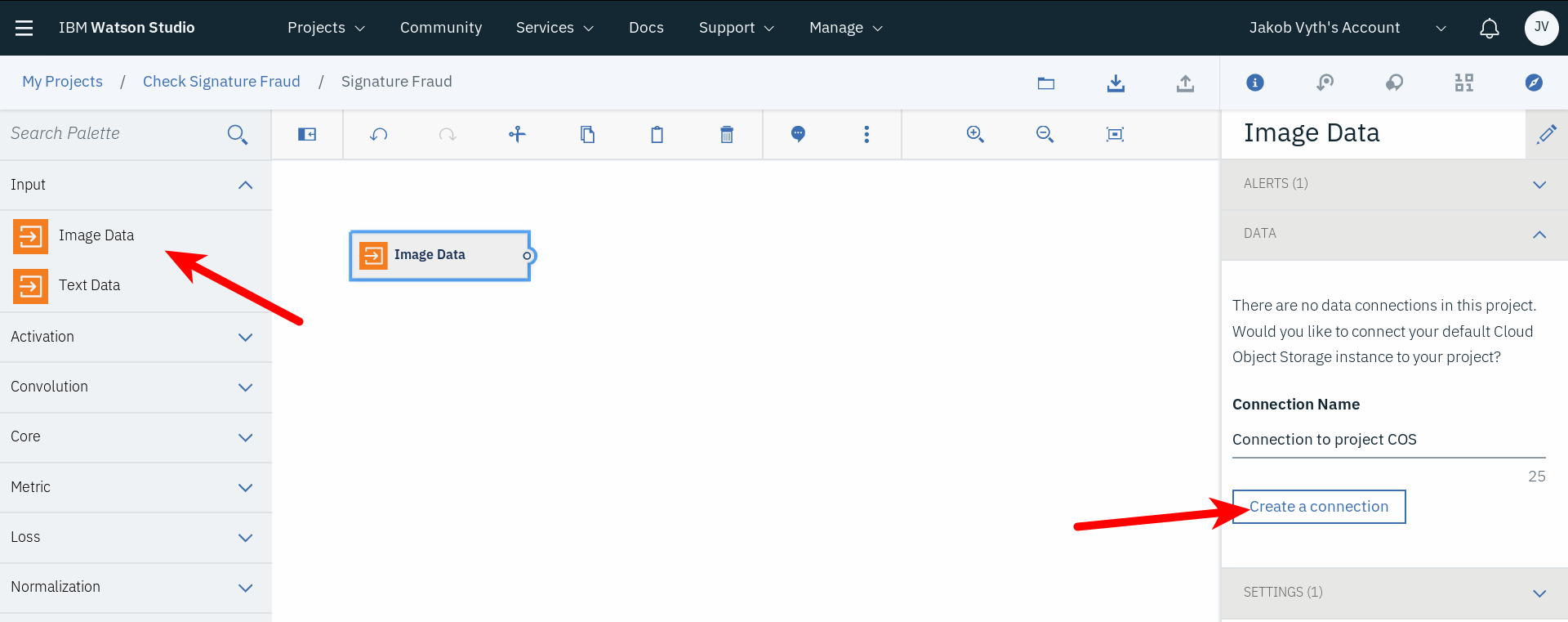
First, we need to provide our neural network with a way to access the data we uploaded earlier. To do this, select an Image Data node from the Input section of the Palette and drag it onto the flow canvas. Double-click the node to modify its properties. In order to define a data source, click Create a connection in the sidebar to the right:
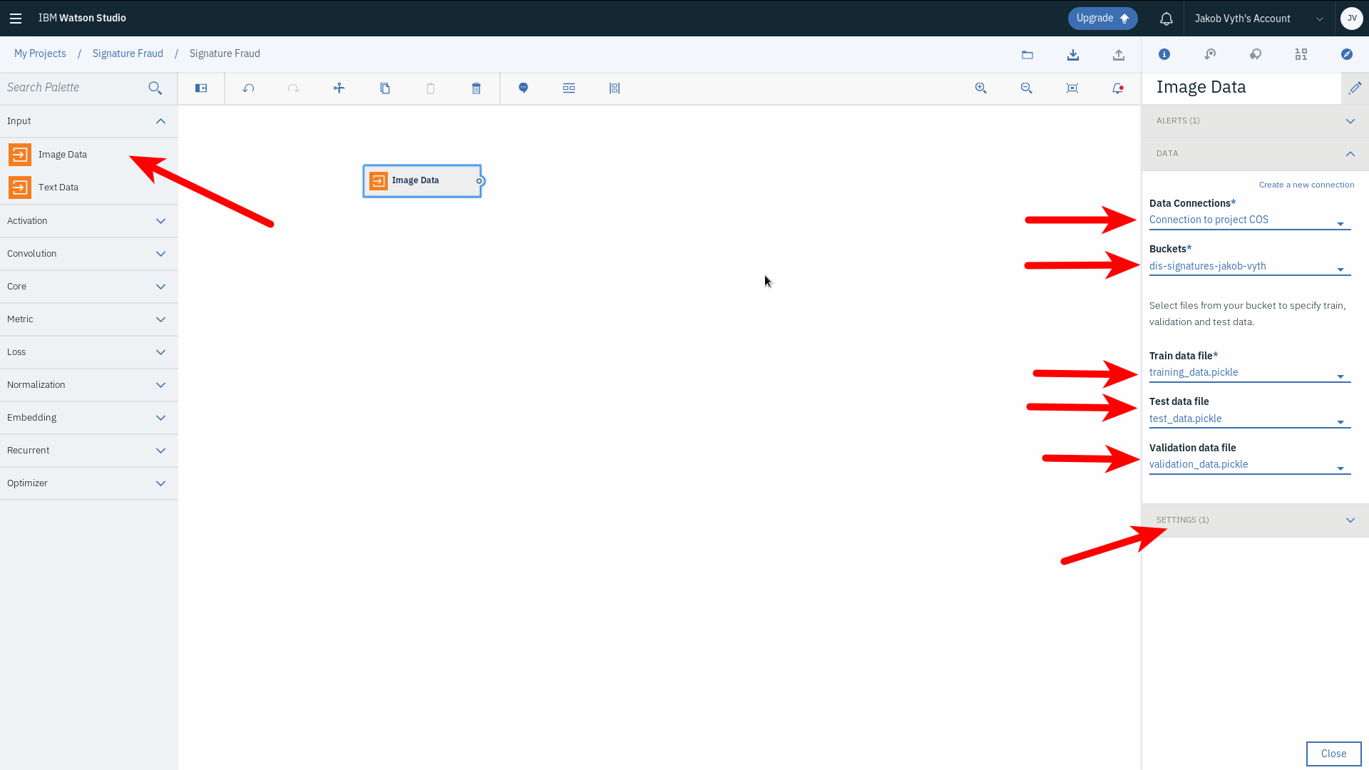
Choose the bucket that contains your data assets. Choose training_data.pickle as the Train data file, test_data.pickle as the Test data file and validation_data.pickle as the Validation data file:
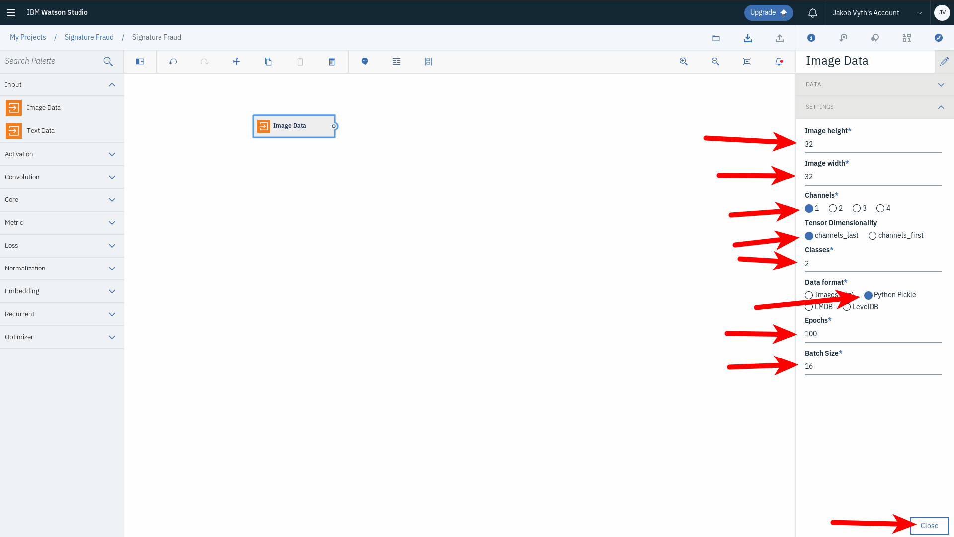
Now close the Data section and switch to the Settings section in the same right-side panel. Adjust all settings as described here and as shown in the screenshot below:
- Set Image height to 32
- Set Image width to 32
- Set Channels to 1 since the images are in grayscale
- Set Tensor dimensionality to channels_last
- Set Classes to 2 since we are trying to classify signature images as either genuine or fraudulent
- Set Data format as Python Pickle
- Set Epochs to 100 (this is how many times the Neural Network will iterate over the data in order to learn more and adjust weights to reach better accuracy)
- Set Batch size to 16 (this is how many images will enter and go through the Neural Network at a time
Once you have all these settings in place, click Close to save them.
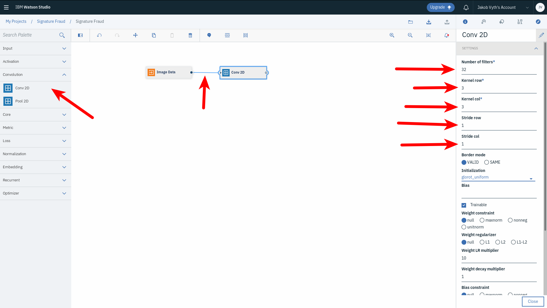
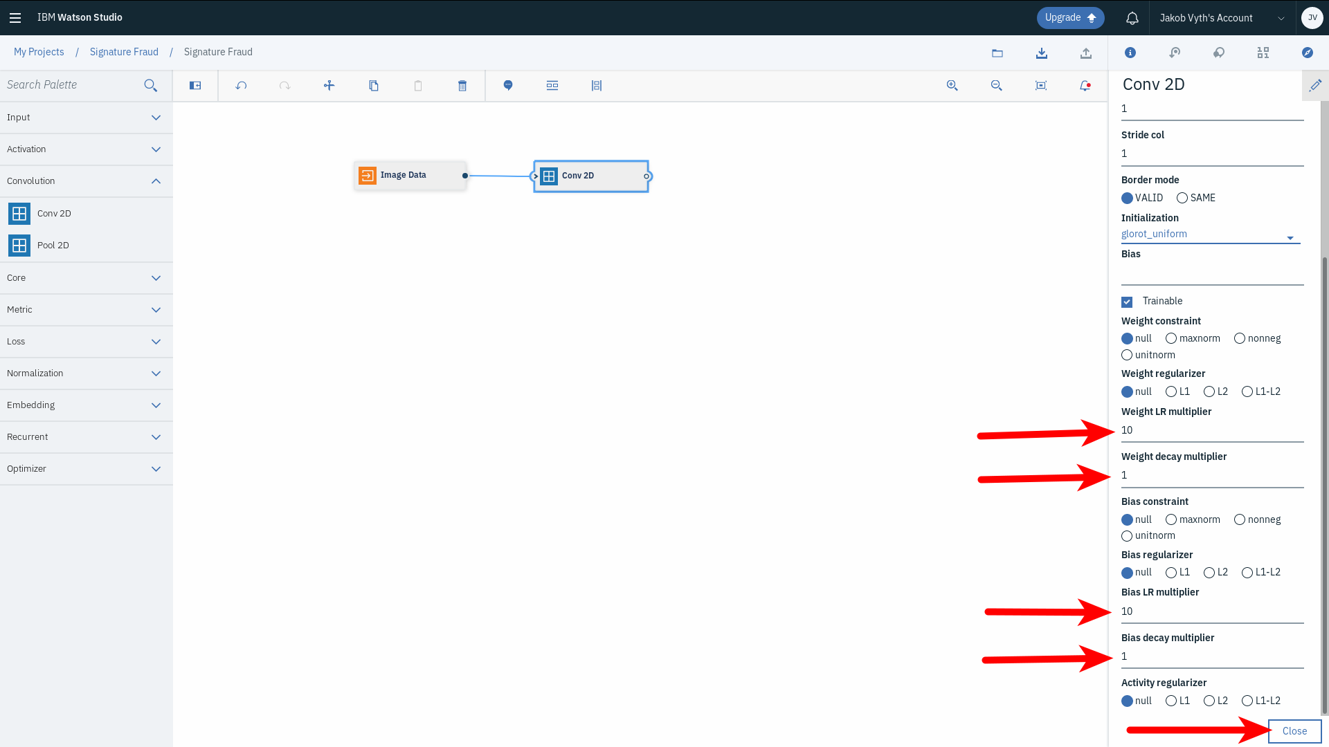
Now let us start building the neural network. The first layer we will add is a 2D Convolutional Layer. Select a Conv 2D node from the Convolution section in the left sidebar and drag and drop it onto the canvas. Connect the two nodes by clicking on the small circle on the right side of the Image Data node and dragging it to the left side circle on the Conv 2D node. Double-click the Conv 2D node to edit its properties. In the right sidebar, change the settings to the following:
- Set Number of filters to 32 (this is the number of feature maps we want to detect in a given image)
- Set Kernel row to 3
- Set Kernel col to 3
- Set Stride row to 1
- Set String col to 1
Continue editing the Conv 2D node properties:
- Set Weight LR multiplier to 10
- Set Weight decay multiplier to 1
- Set Bias LR multiplier to 10
- Set Bias decay multiplier to 1
We only edited the required parameters here. There are other optional parameters that have default settings, such as Initialization, which is the initial weights values. You can set an initial Bias value and set whether it is trainable or not. You can choose a regularization method to minimize overfitting and enhance model generalization. This is a way to penalize large weights and focus on learning small ones as they are lower in complexity and provide better explanation for the data; thus, better generalization for the model.
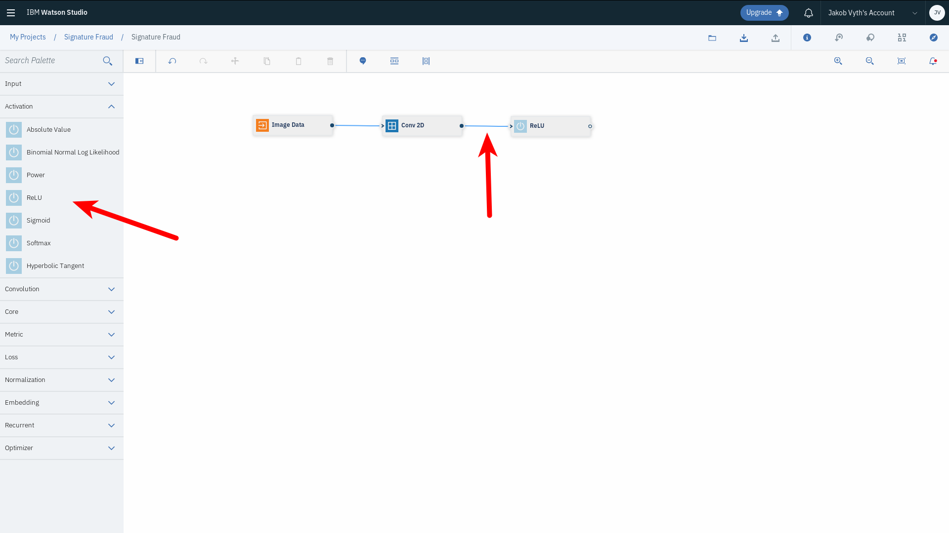
Once you have all the required settings in place, click Close to save them. Next we will add the third node, which is an activation layer. We will choose ReLU (Rectified Linear Unit) as the activation function in our architecture. ReLU gives good results generally and is widely used in Convolutional Neural Networks. Drag a ReLU node from the Activation section in the Palette and drop it onto the canvas. Make sure you are connecting each node to the previous as you create them:
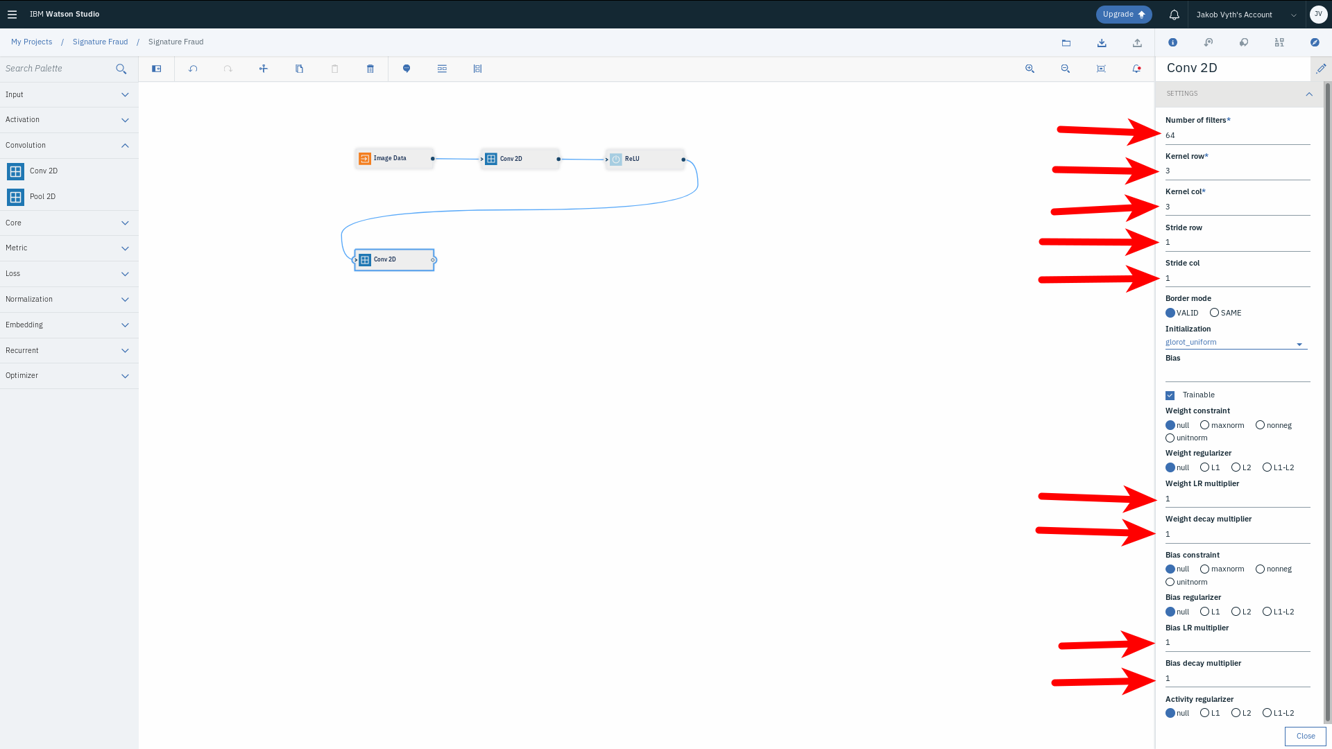
Then, add another Conv 2D layer from the Convolution section. Edit its properties as follows:
- Set Number of filters to 64
- Set Kernel row to 3
- Set Kernel col to 3
- Set Stride row to 1
- Set Stride col to 1
- Set Weight LR multiplier to 1
- Set Weight decay multiplier to 1
- Set Bias LR multiplier to 1
- Set Bias decay multiplier to 1
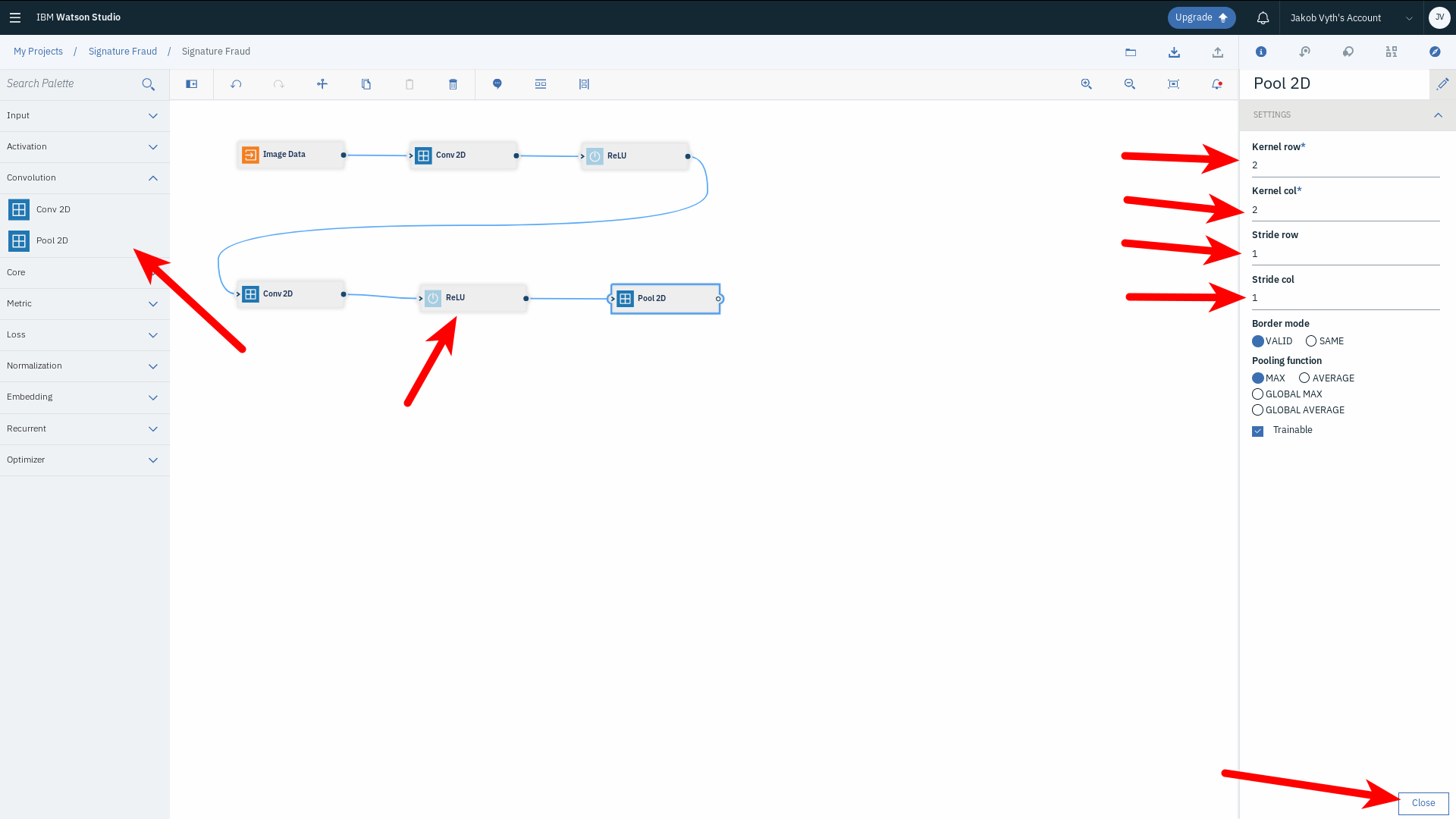
Save these settings by clicking Close. Add another ReLU node from the Activation section. Now, we will add a Max Pooling layer, with the purpose of down-sampling or reducing the dimensionality of the features extracted from the previous convolutional layer. This is achieved by taking the maximum value within specific regions (windows) that will slide across the previous layer’s output. This step helps aggregate many low-level features, extracting only the most dominant ones thus reducing the amount of data to be processed.
Drag and drop a Pool 2D node from the Convolutional section in the sidebar. Double-click it and change its settings:
- Set Kernel row to 2
- Set Kernel col to 2
- Set Stride row to 1
- Set Stride col to 1
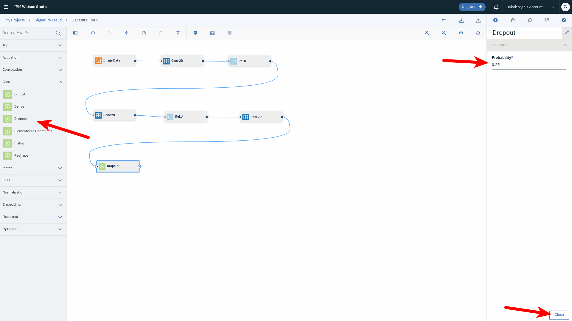
Next up is a Dropout layer. The purpose of this layer is to help reduce overfitting, mainly by dropping or ignoring some neurons in the network randomly. Drag and drop a Dropout node from the Core section. Double-click it, change Probability to 0.25, and click Close.
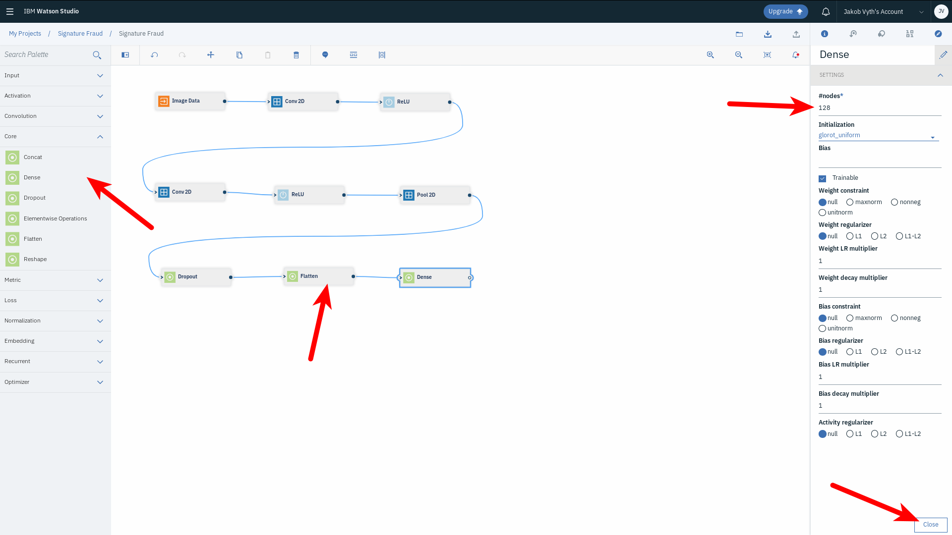
It is time to move on the to the fully connected layers! To do that, we need to flatten the output we have up until now into a 1D matrix. Drag and drop a Flatten node from the Core section. Also drag and drop a Dense node from the Core section. Double-click the Dense node and change #nodes to 128. Click Close.
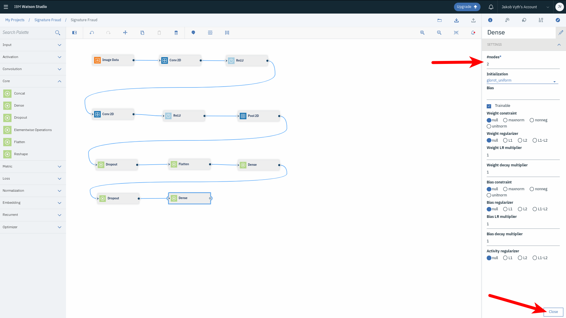
Add another Dropout node from the Core section and change its Probability to 0.5. Click Close. Add a final Dense node. This will represent the output classes (two in this case). Double-click the node and change #nodes to 2 and click Close.
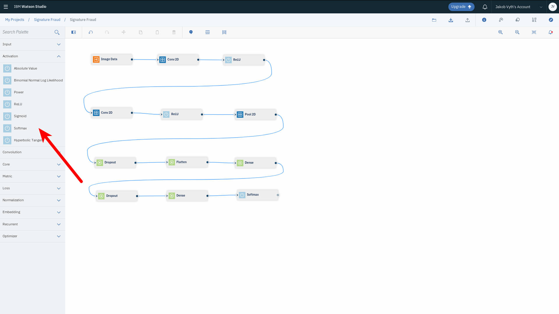
Now, let us add an activation layer at the end of our architecture. We will use Softmax here. It returns an output in the range of [0, 1] to represent true and false values for each node in the final layer.
Drag and drop a Softmax node from the Activation section.
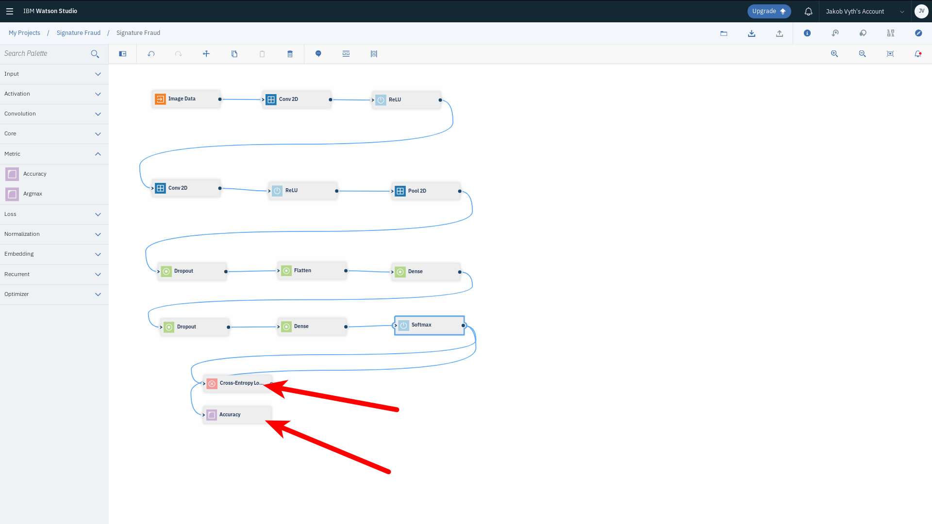
We will need to add some means of calculating the performance of the model. This is represented in the form of a cost function, which calculates the error of the model's predicted outputs in comparison to the actual labels in the dataset. Our goal is to minimize the loss as much as possible. The function we will use is Cross-Entropy. We will also add another node to calculate the accuracy of our model’s predictions.
Drag and drop a Cross-Entropy node from the Loss section, and an Accuracy node from the Metrics section. Connect them both to the Softmax node:
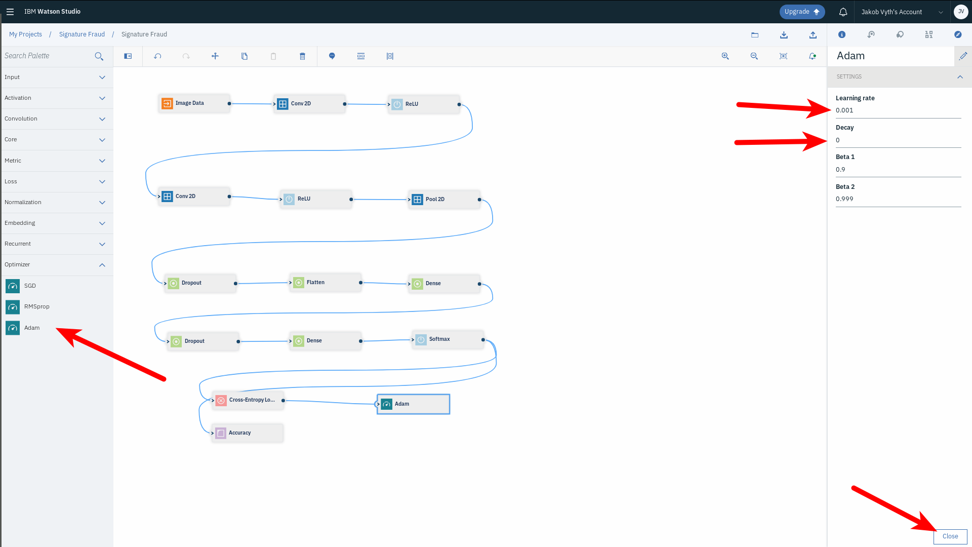
Finally, we will add an optimization algorithm which defines how the model will fine tune its parameters to minimize loss. There are many such algorithms, but we will use an Adam optimizer as it is a generally well-functioning optimization algorithm. Drag and drop an Adam node from the Optimizer section. Double-click it and change its settings:
- Set the Learning rate to 0.001
- Set the Decay to 0 (with an Adam optimizer, we do not need to set this value as Adam does not make use of it)
Connect the Adam node to the Cross-Entropy node:
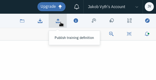
Now that we have the full architecture of our Neural Network, let us start training it and see how it performs on our dataset. You can do that directly from Watson Studio’s Neural Network Modeler’s interface. In the top toolbar, select the Publish training definition tab and click it:
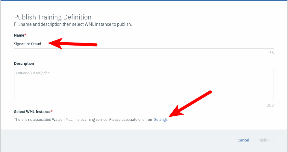
Name your model so you can identify it later. You will need to have a Watson Machine Learning Service associated to your project. If one is not associated already, you will be prompted to do that on the fly. In the given prompt, click the Settings link:
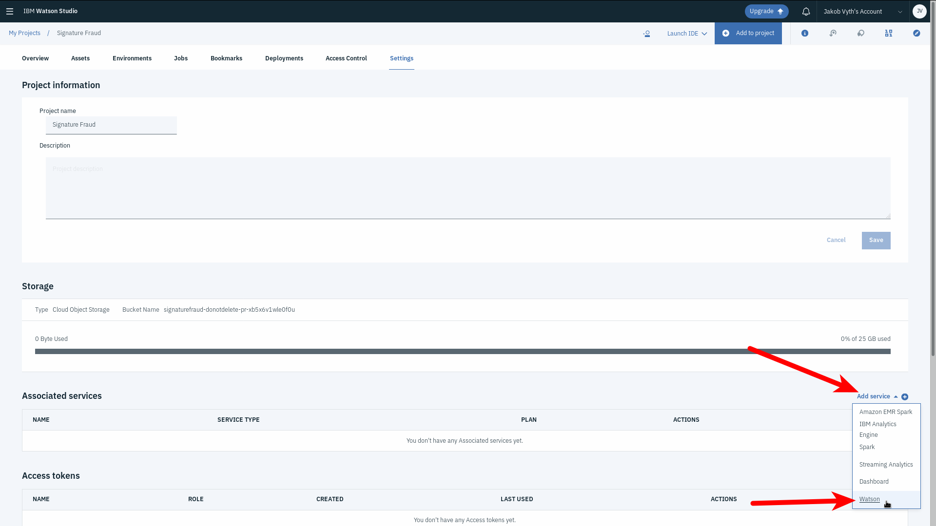
You will be redirected to the project settings page. Here you can manage all services and settings related to your current project. Scroll down to the Associated Services section, click Add service and select Watson from the drop-down menu:
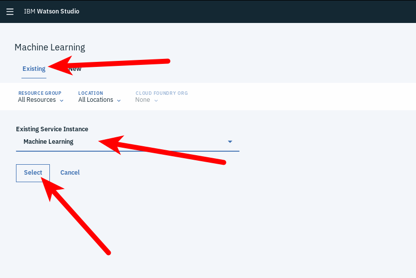
You will then be presented with all available Watson services. Choose Machine Learning and click Add. Select your Machine Learning service instance and click Select:
This will redirect you back to the project settings page. Click on Assets and scroll down to the Modeler flows section. Click on the flow we have been working on.
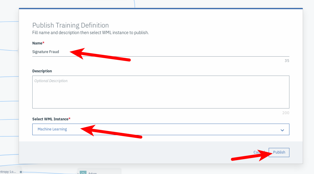
Once your flow loads, again click on the Publish training definition tab. Make sure that your model is named and that the Machine Learning service is detected and selected, then click Publish:
When the training definition has been published, you will find a notification at the top of the screen showing you a link to train the model in Experiments. Click it:
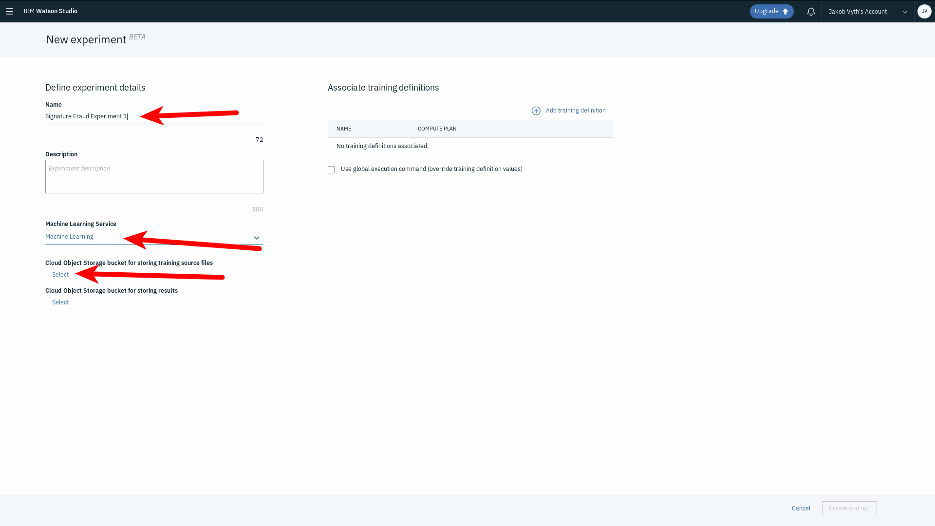
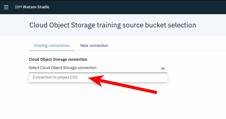
We will now create a new Experiment. Start by giving it a name, then select the Machine Learning service. Lastly, we need to define the source of our data and where we will store the training results. Choose the bucket containing your dataset by clicking Select:
From the drop-down menu, choose your already existing Object Storage connection:
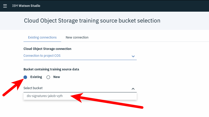
Choose the correct bucket by marking the Existing radio button and selecting the name of the bucket where you saved the dataset. Click the Select button at the bottom of the page:
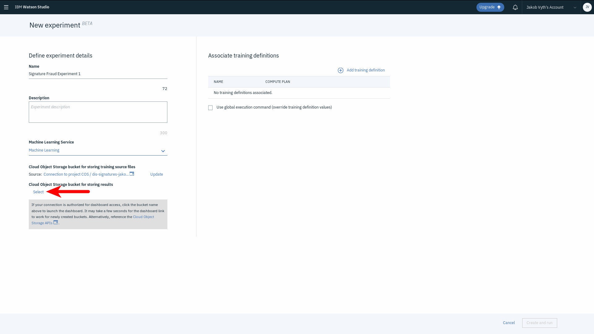
You will be redirected back to the new Experiment form to choose where to store your training results. Click Select:
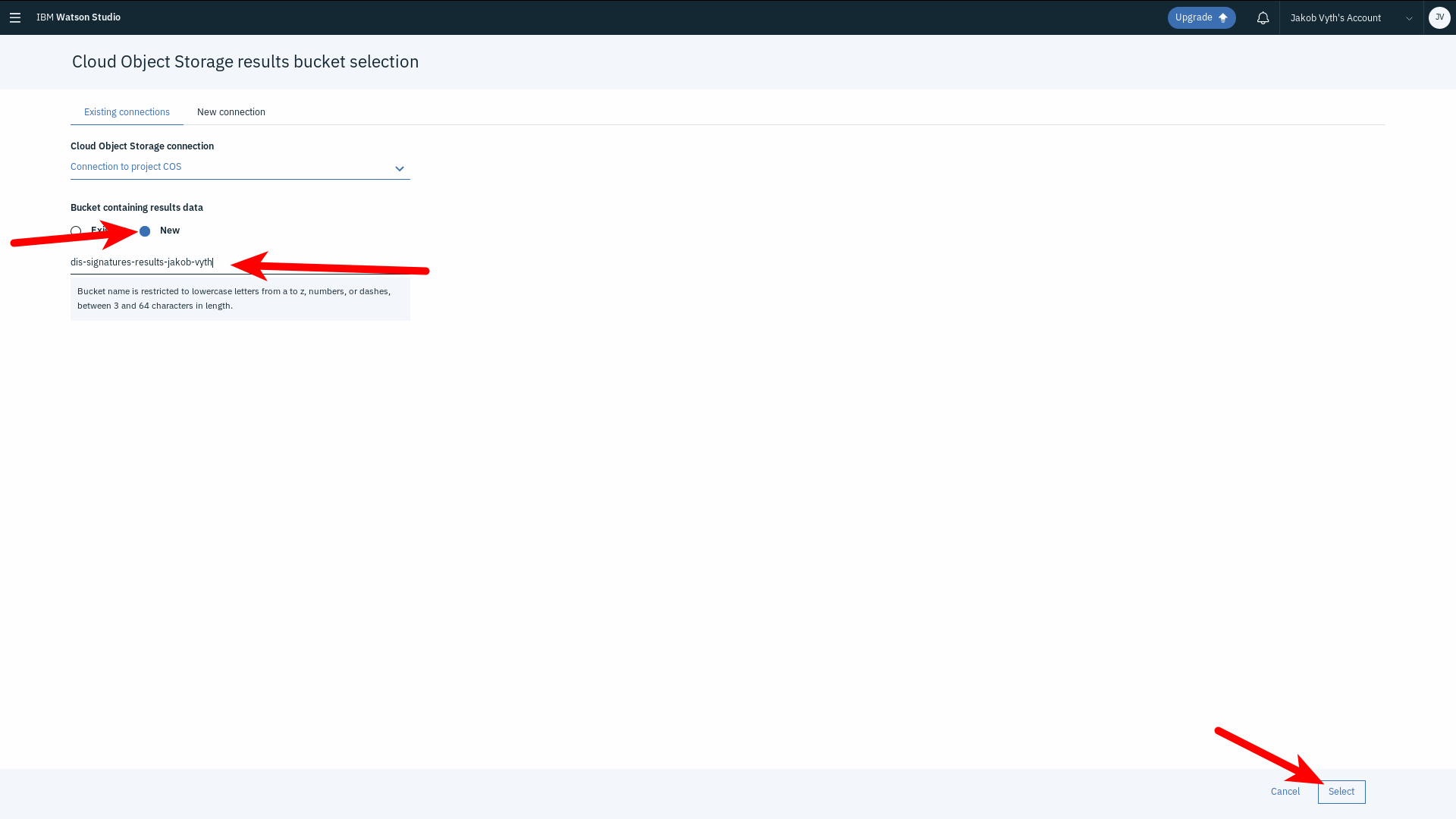
Like before, choose Existing connection and select your Object Storage connection from the drop-down. Now, however, mark the New radio button and give your new results bucket a name (remember that buckets must have globally unique names!):
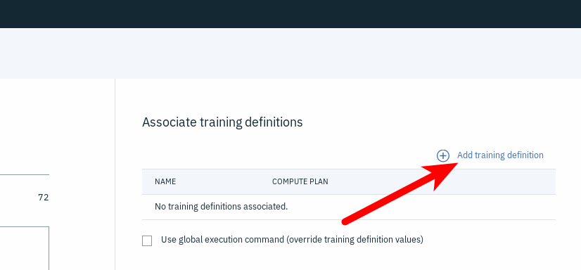
Click Select to return the the new Experiment form. Click Add training definition:
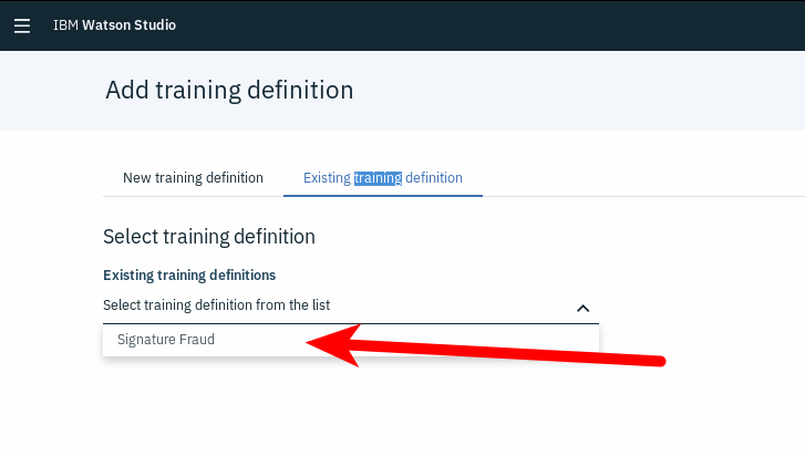
Since we already published a training definition from Neural Network Modeler, we will select the Existing training definition option:
From the drop-down, select the training definition we created:
Now we have to select the hardware that will be used to train the model. Choose 1/2 x NVIDIA Tesla K80 (1 GPU) from the drop-down (should be the first option). For the Hyperparameter Optimization Method, select None:
Finally, click Select in the bottom right corner. Back to the new Experiment form for the last time. At this point, everything should be set. Click Create and run at the bottom of the page to start training your model!
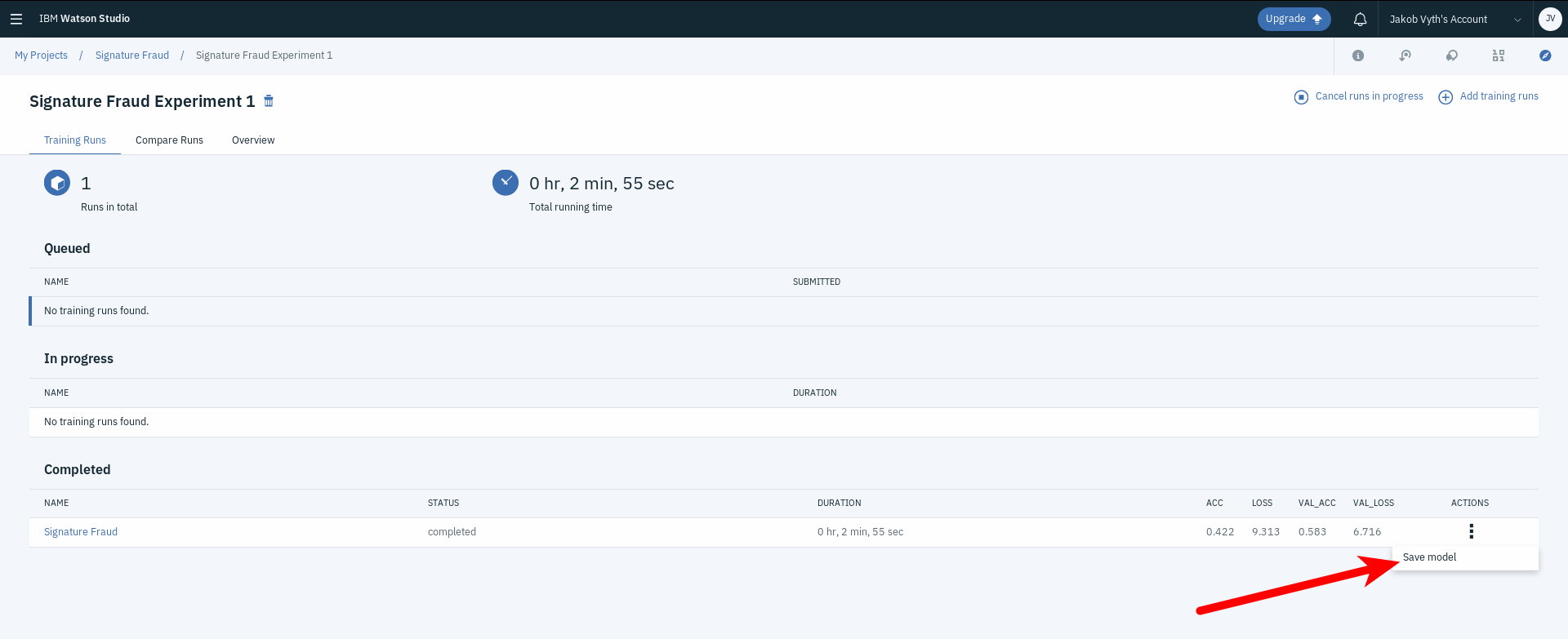
You will be presented with a view with details about the process. Once your model is trained (should take a couple of minutes), it will be listed in the Completed section at the bottom of the page.
Click the three vertical dots under the Actions tab and select Save Model:
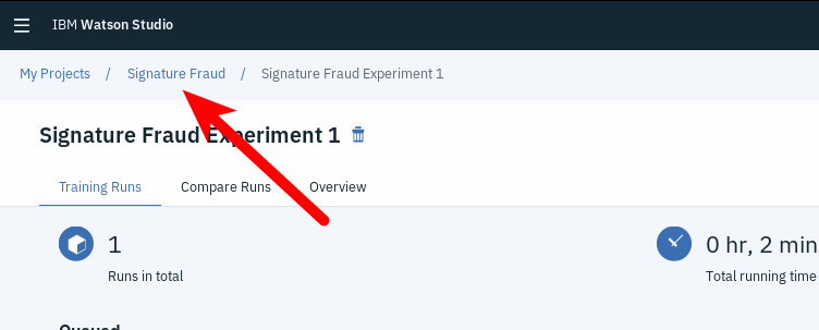
Give your model a name, save it, then make your way back to the project dashboard by clicking on your project name:
Under Models, click on the model you just saved and navigate to the Deployments tab. Click Add Deployment:
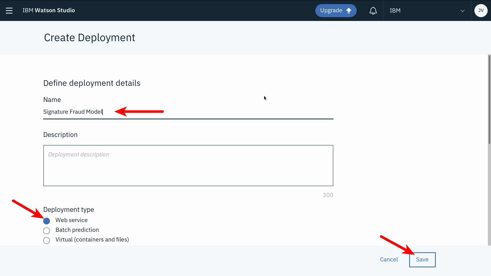
Give your deployed model a name, make sure the Web service radio button is marked, and click Save:
The STATUS field will tell you when the model has been successfully deployed:
Your model is now ready to score images via API calls!
Now it is time to call your model's API and let it score an image of a fraudulent signature! The signature we will score is this one:
The reason that it is blurred like it is, is that it has to be converted to 32x32 pixels grayscale before it can be scored by the neural network model.
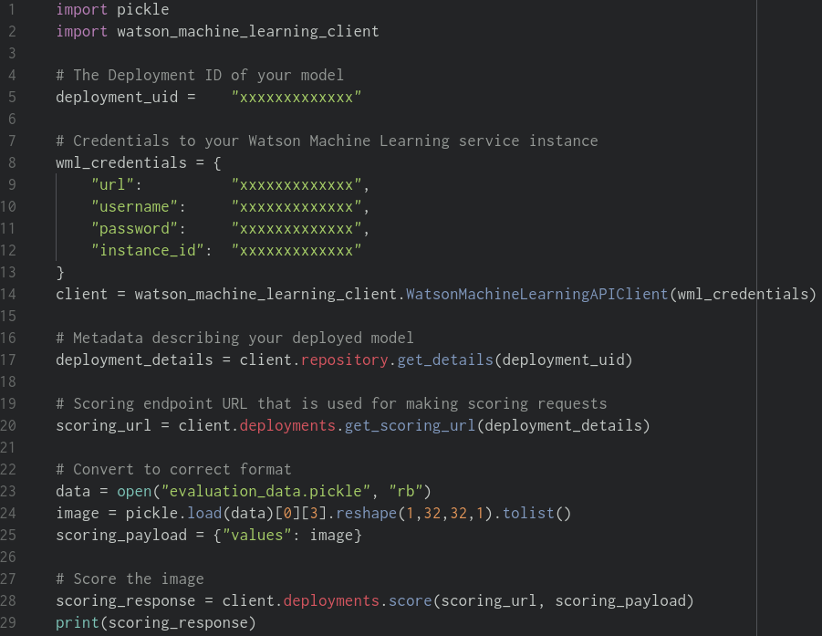
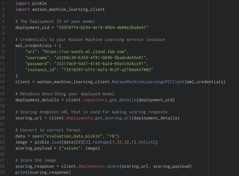
First, examine the python file that was included in the zipped assets by opening evaluate.py using your favorite text editor. This file contains (almost) everything needed to call your model's API:
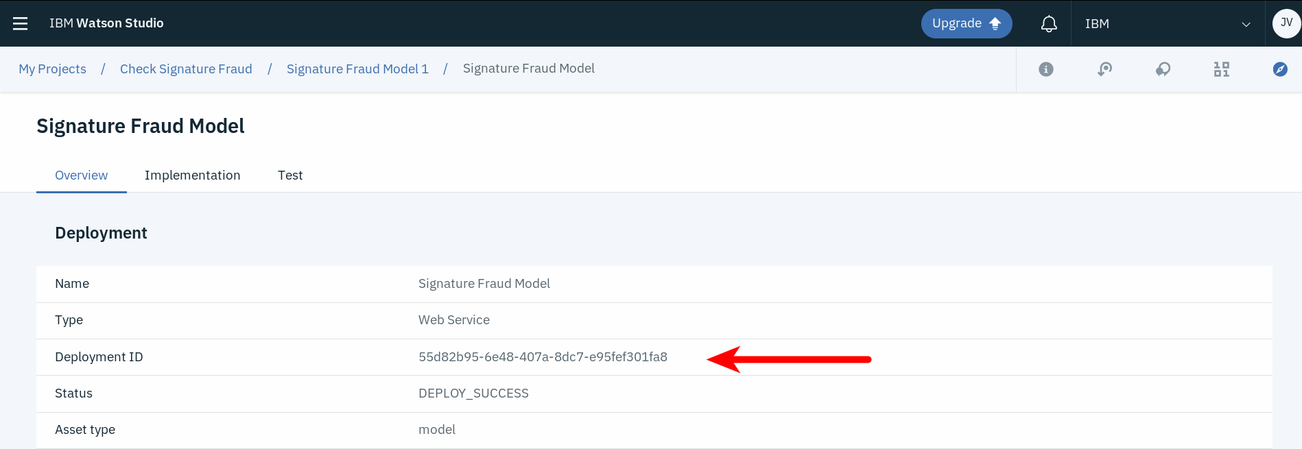
As you can see, the values for deployment_id, url, username, password, and instance_id are missing! Before we can call the model, we need to gather these bits of data. First up: deployment_id. Go to your project dashboard and click the Deployments tab, then click on your deployed model:
deployment_id should be right there. Copy and paste it inside the string literals in the evaluate.py file.
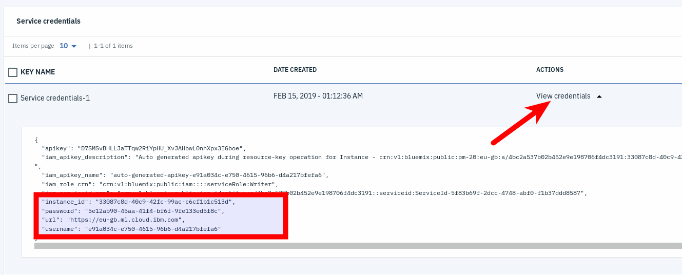
Next up: the rest. url, username, password, and instance_id are all used to identify yourself when calling the API. In order to find them, you must go to the main IBM Cloud dashboard and find your Machine Learning service instance:
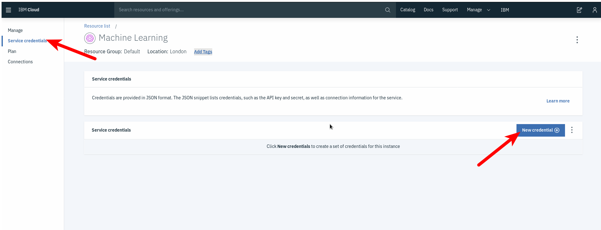
Click it and navigate to the Service credentials tab. Click New credential:
Leave everything as-is and click Add.
Access your newly made credentials by clicking View credentials under the Action field. This is where we can find the information we need!
Copy the values of url, username, password, and instance_id into the correct places in evaluate.py. The end result should look very similar to this:
You are now ready to run the file and let you model score an image! Using whatever tool you want to run the evaluate.py file. You should get a printout looking like this if your model if your model correctly identified the model as fraudulent:
Or this, if your model did not identify it as fraudulent:
In this tutorial, you learned about the powerful deep learning tools available in Watson Studio. You learned how to quickly prototype a neural network architecture using the Neural Network Modeler. You learned how to publish the Neural Network Flow and train it using Experiments. You also learned how to deploy your model and how to call its API to let it score an image using the Watson Machine Learning Python SDK.
