Python library implementing some Evolutionary Algorithms. These follow an ask/tell work flow where one:
- new trial members/sample are requested using ask(), these need to me manually evaluated,
- the fitness socores are then fed back to the object with tell() to enable a population update. This structure enables the code to be used simply with any model.
Current features include:
- Three EAs (DE, OpenAI-ES, CMAES)
- Page Trend test for convergence statistical analysis
Differential Evolution (DE) is an easily implemented and effective optimisation algorithm for exploiting real-world parameters. DE is a derivative-free, stochastic, population-based, heuristic direct search method [1] which only requires a few robust control variables.
A simple work flow might be:
from pyeas import DE

# call object passing in hyperparameters and bounderies for each optimisable parameter
optimizer = DE(mut=0.6,
               crossp=0.6,
               bounds=np.array([[-5,5],[-5,5]]),

for generation in range(num_gens):

    # ask for a trial population
    trial_pop = optimizer.ask(loop=generation)

    # Loop through trial pop and evaluate their fitnesses
    solutions = []
    for trial in trial_pop:
        fitness = f(trial)
        solutions.append((value))

    # Tell the object the evaluated values.
    optimizer.tell(solutions, trial_pop)
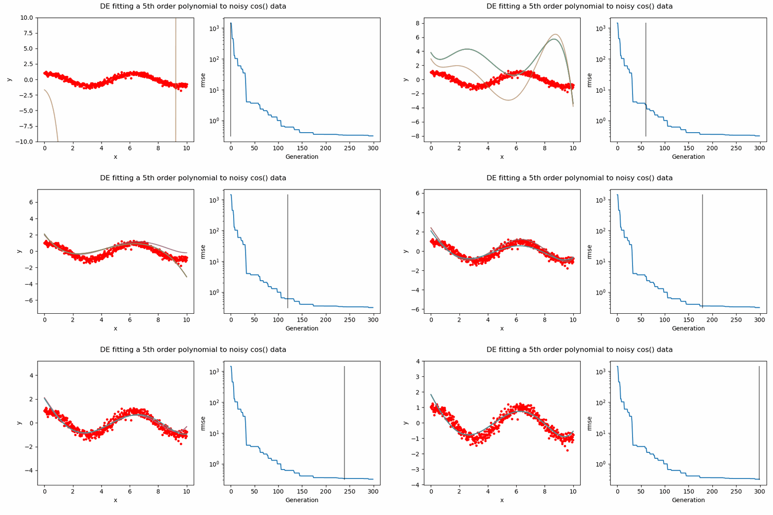
An Example of DE/best/1/bin solving some simple problems, as generated by eg_funcs.py:
An example of DE/ttb/1/bin solving a 5th order polynomial to fit noisy cos(x) data.
Evolutionary Strategies (ES) involve the evaluation of a population of real valued genotypes (or population members), after which the best members are kept, and others discarded.
Natural Evolutionary Strategies (NES) are a family of Evolution Strategies which iteratively update a search distribution by using an estimated gradient on its distribution parameters. Notably, NES performs gradient accent along the natural gradient.
The OpenAI Evolutionary Stratergy (OAIES) algorithm is a type of NES [2], implemented here as vanilla gradient decent, with momentum, or with adam optimiser [3].
A simple work flow might be:
from pyeas import OAIES

# call object passing in hyperparameters and bounderies for each optimisable parameter
optimizer = OAIES(alpha=0.01,
                 sigma=0.002,
                 bounds=np.array([[-10,10],[-10,10]]),
                 population_size=20,
                 optimiser = 'adam',
                 seed=1)

for generation in range(num_gens):

    # ask for a pseudo-population
    trial_pop = optimizer.ask(loop=generation)

    # Loop through pseudo-pop and evaluate their fitnesses
    solutions = []
    for trial in trial_pop:
        fitness = f(trial)
        solutions.append((value))

    # Tell the object the evaluated values.
    optimizer.tell(solutions, trial_pop)

    # Calc the new parent fitness, and tell again!
    parent_fit = f(optimizer.parent)
    optimizer.tellAgain(parent_fit)
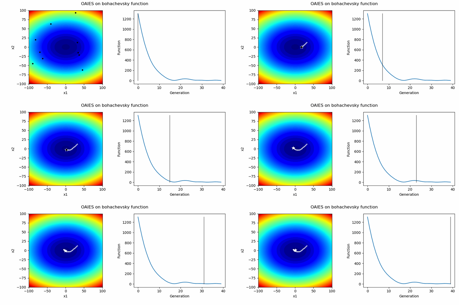
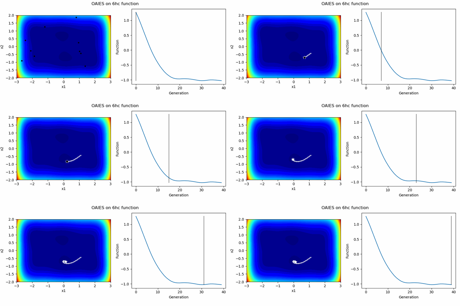
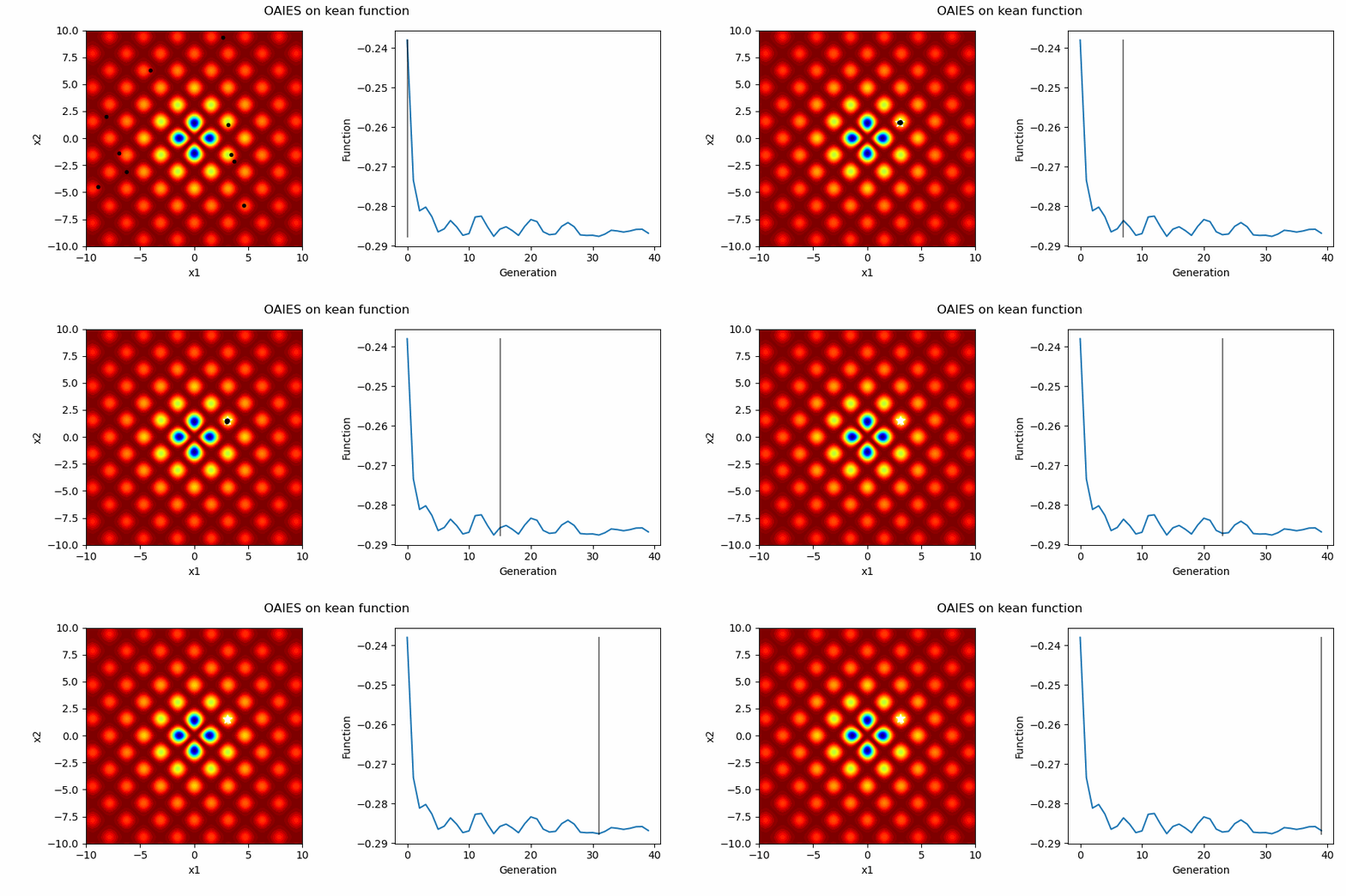
An Example of OAIES solving some simple problems, as generated by eg_funcs.py:
The Covariance Matrix Adaptation Evolution Strategy (CMAES) algorithm is a popular stochastic method for real-parameter (continuous domain) optimization [4]. In the CMAES, a population of new search points is generated by sampling a Multivariate Gaussian Distribution (MGD), fitness results are then used to update and adapt the MGD.
A simple work flow might be:
from pyeas import OAIES

# call object passing in hyperparameters and bounderies for each optimisable parameter
optimizer = CMAES(start='mean',
                  sigma=0.002,
                  bounds=np.array(bound),
                  seed=2)

for generation in range(num_gens):

    # ask for a pseudo-population
    trial_pop = optimizer.ask()

    # Loop through pseudo-pop and evaluate their fitnesses
    solutions = []
    for trial in trial_pop:
        fitness = f(trial)
        solutions.append((value))

    # Tell the object the evaluated values.
    optimizer.tell(solutions, trial_pop)

    # Calc the new parent fitness, and tell again!
    parent_fit = f(optimizer.parent)
    optimizer.tellAgain(parent_fit)
This implementation of CMAES can have its starting location as either:
- A passed in array denoting starting values
- The mean of the boundaries ('mean')
- A random initital population used to select a good starting point ('random')
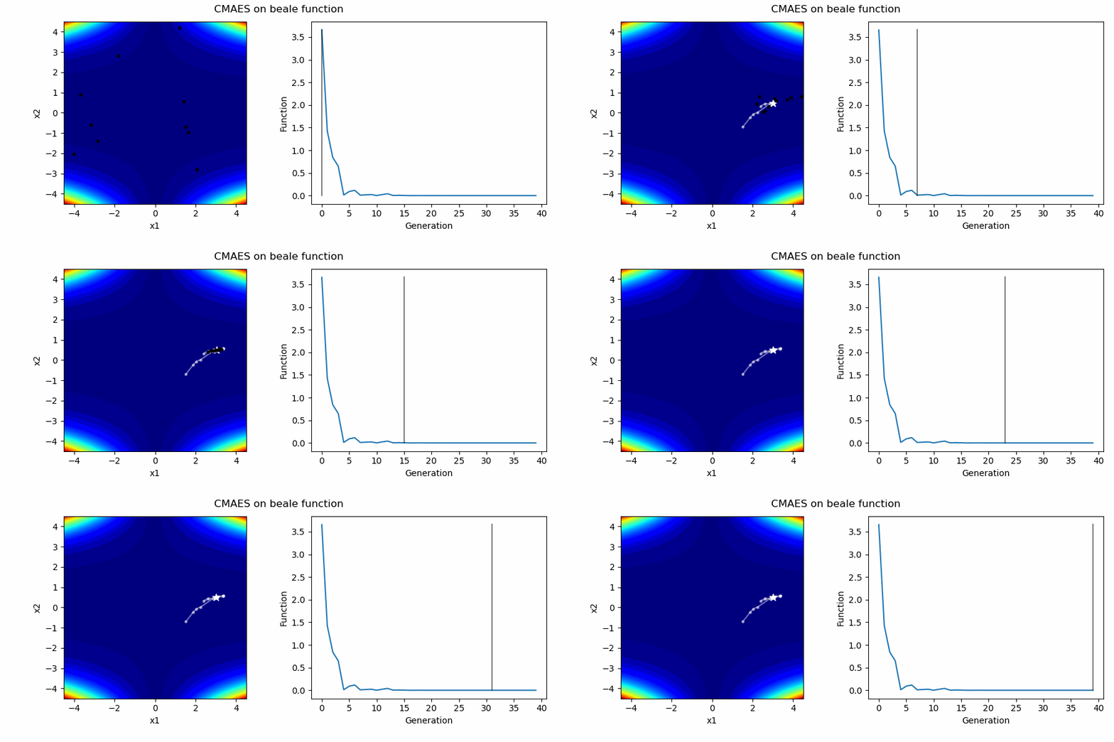
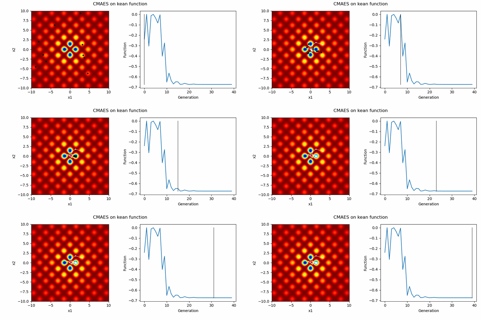
An Example of CMAES solving some simple problems (with random starting locations), as generated by eg_funcs.py:
We can notice that different hyperparameter values might result in wildly different convergence speeds per amount of evaluations/computations executed. In cases where completing an evaluation is computationally expensive, ideally the algorithm should provide meaningful generational updates while only requiring a minimal number of evaluations in that generation [5].
Consider how we might set a maximum number of computations/evaluations limit (e.g., for the DE algorithm):
optimizer = DE(mut=0.6,
               crossp=0.6,
               bounds=np.array([[-5,5],[-5,5]]),

 # Break after set number of computations (i.e., evaluations)
while optimizer.evals < max_ncomps:

    # ask for a trial population
    trial_pop = optimizer.ask(loop=generation)

    # Loop through trial pop and evaluate their fitnesses
    solutions = []
    for trial in trial_pop:
        fitness = f(trial)
        solutions.append((value))

    # Tell the object the evaluated values.
    optimizer.tell(solutions, trial_pop)
We can then use this to consider fairer comparisons between alorithms.
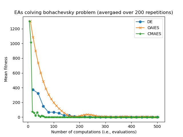
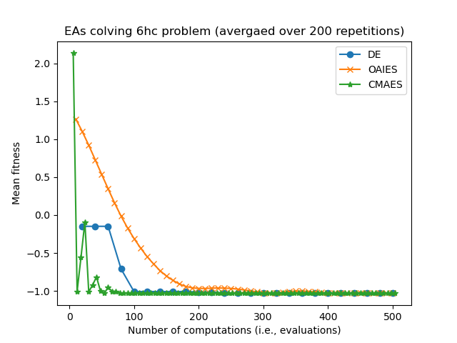
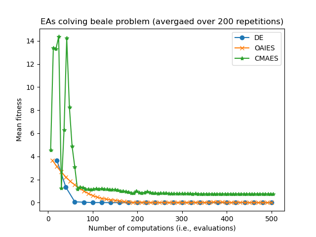
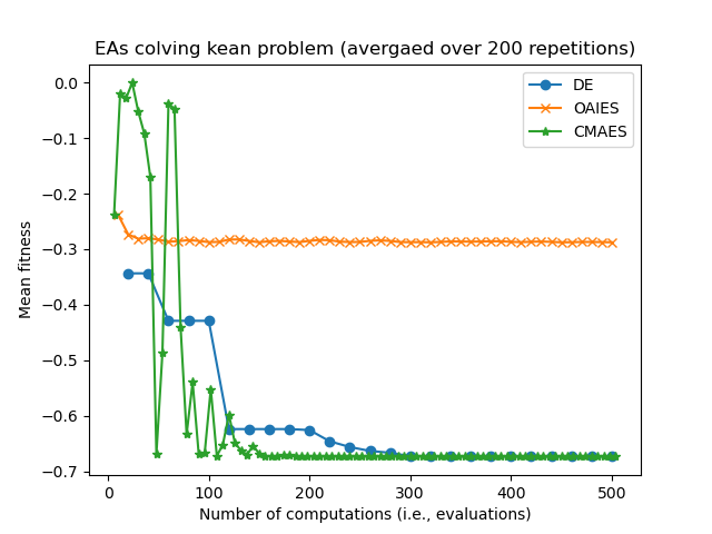
Consider some results from eg_funcs_ncomps.py showing the mean parent fitness covergence:
Notice how CMAES and OAIES can have fitnesses which go up and down, unlike the fitnesses of the DE parent(s) which can only ever decrease.
Also notice how CMAES has many more generational updated in the allotted 500 computations/evaluations, where as the DE algorithm has fewer generational updates since (in this example) the population size is set much larger. we are now in the realm of hyperparamater tuning...
Finnaly, to actually do a statisitcal test and compare EA convergence, we can use the page trend test [6], implemented here.
We also address the posability that two algorithms might have different x-axis values (as in the previous section). An example is given in eg_PageTest_interp.py.
You might not always want a population member to be a 1d array with a corresponding boundary array. e.g.,
- member: [-0.5, -1.9, 1.6, -2, 8],
- boundaries: [ [-1,1], [-2,2], [-2,2], [-10,10], [-10,10] ]
Instead, we might want to group a member into sub arrays corresponding to a list of boundaries. We can do this using the 'groupings' argument. e.g.,
- member: [[-0.5], [-1.9, 1.6], [-2, 8]],
- boundaries: [ [-1,1], [-2,2], [-10,10] ]
- grouping: [1, 2, 2]
[1] R. Storn and K. Price, “Differential Evolution – A Simple and Efficient Heuristic for global Optimization over Continuous Spaces,” Journal of Global Optimization, vol. 11, no. 4, pp. 341–359, Dec. 1997. [Online]. Available: https://doi.org/10.1023/A:1008202821328
[2] T. Salimans, J. Ho, X. Chen, S. Sidor, and I. Sutskever, “Evolution Strategies as a Scalable Alternative to Reinforcement Learning,” Sep. 2017. [Online]. Available: http://arxiv.org/abs/1703.03864
[3] D. P. Kingma and J. Ba, “Adam: A Method for Stochastic Optimization,” arXiv, Jan. 2017. [Online]. Available: http://arxiv.org/abs/1412.6980
[4] Hansen, N. (2016). The CMA Evolution Strategy: A Tutorial. Available: https://arxiv.org/abs/1604.00772
[5] Benedict. A. H. Jones, N. Al Moubayed, D. A. Zeze, and C. Groves, ‘Enhanced methods for Evolution in-Materio Processors’, in 2021 International Conference on Rebooting Computing (ICRC), Nov. 2021, pp. 109–118. http://doi.org/10.1109/ICRC53822.2021.00026.
[6] Derrac, J., Garc ́ıa, S., Hui, S., Suganthan, P. N., and Herrera, F. (2014). Analyzing con- vergence performance of evolutionary algorithms: A statistical approach. Information Sciences, 289:41–58. http://dx.doi.org/10.1016/j.ins.2014.06.009


