csatimer

csatimer provides data on how much airtime French politician receive in the media.

The datasets contained in the package are also available in the csv-format.

Installation

# install.packages("devtools")
devtools::install_github("benjaminguinaudeau/csatimer")

Data

Last Update: February, 2nd 2022

Two types of datasets are provided:

speaking time of politicians during routine period (no electoral campaigns)
speaking time of candidates during political campaigns

Routine period (no electoral campaigns)

Every month, the CSA collects how long each political personality speaks on each of the major radio and TV stations.

This dataset can be accessed using read_csa_routine and is continuous between September 2017 and January 2022.

read_csa_routine() %>%
  glimpse
#> Rows: 109,068
#> Columns: 7
#> $ month     <date> 2017-09-01, 2017-09-01, 2017-09-01, 2017-09-01, 2017-09-01,…
#> $ station   <chr> "TF1", "France 2", "France 2", "France 2", "France 2", "Fran…
#> $ prog_type <chr> "JT", "JT", "JT", "MAG", "MAG", "PROG", "JT", "MAG", "JT", "…
#> $ name      <chr> "Macron Emmanuel", "Macron Emmanuel", "Macron Emmanuel", "Ma…
#> $ label     <chr> "Président De La République En Débat Politique", "Président …
#> $ party     <fct> "Exécutif", "Exécutif", "Exécutif", "Exécutif", "Exécutif", …
#> $ time      <dbl> 8.416667, 7.933333, 4.050000, 6.300000, 2.266667, 3.500000, …

It contains the following columns:

month "2017-01-01"
station "TF1", "France 2", "France Inter", ...
prog_type "JT", "MAG", "PROG"
name "Emmanuel Macron", "Marine Le Pen", "François Hollande", ...
label "Président", "Parti Socialiste", "Ministre", "Les Républicains", ...
party "Exécutif" , "Ps", "LR", ...
time

Speaking times are measured in minutes. For instance, in September 2017, Emanuel Macron spoke 8.4 minutes on TF1.

prog_type refers to different types of TV/Radio shows:

JT: newscast
MAG: political shows
PROG: non-political shows

Electoral campaigns

During electoral campaigns - presidential, legislative and local - , the CSA publishes airtime of campaigning candidates data every two weeks.

For each candidate, three different measures are computed:

time_candidat: speaking time of the candidate themselves
time_support: speaking time of personalities supporting the candidate
time_mention: speaking time of journalists mentioning the candidate

This dataset can be accessed using read_csa_election("pres_2022").

Following elections are available:

Presidential elections 2022: read_csa_election("pres_2022")
Presidential elections 2017: read_csa_election("pres_2017")

read_csa_election("pres_2022")  %>%
  dplyr::glimpse()
#> Rows: 265
#> Columns: 9
#> $ type          <chr> "presidential", "presidential", "presidential", "preside…
#> $ constituency  <chr> "national", "national", "national", "national", "nationa…
#> $ date_start    <date> 2022-01-01, 2022-01-01, 2022-01-01, 2022-01-01, 2022-01…
#> $ date_end      <date> 2022-01-16, 2022-01-16, 2022-01-16, 2022-01-16, 2022-01…
#> $ station       <chr> "BFM", "BFM", "BFM", "BFM TV", "BFM TV", "BFM TV", "BFM …
#> $ candidat      <chr> "Macron Emmanuel", "Pecresse Valerie", "Zemmour Eric", "…
#> $ time_candidat <dbl> 0.0000000, 0.1333333, 0.6000000, 9.7166667, 50.9166667, …
#> $ time_support  <dbl> 3.9833333, 0.0000000, 0.0000000, 0.0000000, 31.0500000, …
#> $ time_mention  <dbl> 0.0000000, 0.0000000, 1.3166667, 0.0000000, 3.0666667, 1…

Updating data

Data will be updated as the CSA publishes new routine and campaign data.

To update the data local version, use update_csatimer()

# Updating data
update_csatimer()
#> ℹ Updating 2017
#> ℹ Updating 2018
#> ℹ Updating 2019
#> ℹ Updating 2020
#> ℹ Updating 2021
#> ℹ Updating pres_2017
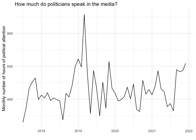
#> ℹ Updating pres_2022

Example

Here are some graphic examples using csatimer::read_csa_routine()

Example 1

read_csa_routine() %>%
  group_by(month) %>%
  summarise(n_hours = sum(time, na.rm = T)/60) %>%
  ggplot(aes(x = month, n_hours)) +
  geom_line() +
  theme_minimal() +
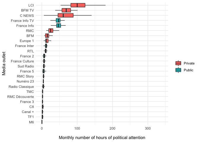
  labs(x = "", y = "Monthly number of hours of political attention", title = "How much do politicians speak in the media?")

Example 2

read_csa_routine() %>%
  add_station_dummies %>%
  mutate(private = ifelse(is_private, "Private", "Public")) %>%
  group_by(private, station, month) %>%
  summarise(n_hours = sum(time, na.rm = T)/60) %>%
  ungroup %>%
  mutate(station = fct_reorder(station, n_hours)) %>%
  ggplot(aes(x = station, n_hours, fill = private)) +
  geom_boxplot(outlier.alpha = 0) +
  coord_flip() +
  labs(x = "Media outlet", y = "\nMonthly number of hours of political attention", fill = "") +
  theme_minimal() 
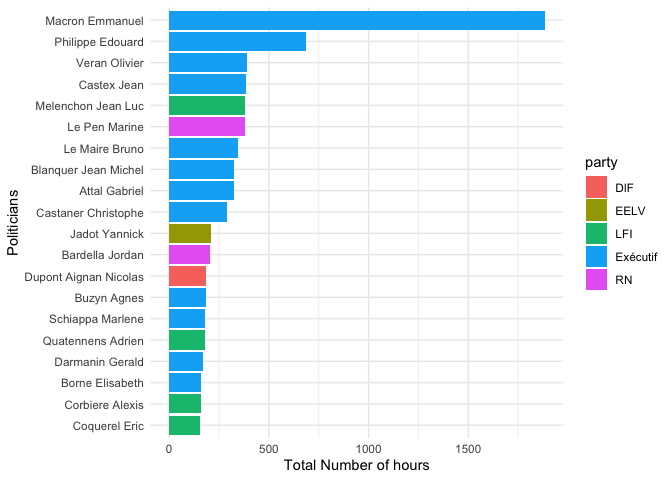
#> `summarise()` has grouped output by 'private', 'station'. You can override using the `.groups` argument.

Example 3

read_csa_routine() %>% 
  group_by(party, name) %>%
  summarise(n_hours = sum(time, na.rm = T)/60) %>%
  ungroup %>%
  slice_max(n_hours, n = 20) %>%
  mutate(name = fct_reorder(name, n_hours)) %>%
  ggplot(aes(x = name, y = n_hours, fill = party)) +
  geom_col() +
  coord_flip() +
  theme_minimal() +
  labs(x = "Politicians", y = "Total Number of hours")
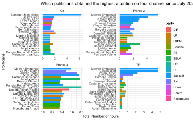
#> `summarise()` has grouped output by 'party'. You can override using the `.groups` argument.

Example 4

read_csa_routine() %>% 
  filter(month > lubridate::dmy("07-01-2021")) %>%
  filter(station %in% c("TF1", "France 2", "France 3", "C8")) %>%
  group_by(station, party, name) %>%
  summarise(n_hours = sum(time, na.rm = T)/60) %>%
  ungroup %>%
  group_by(station) %>%
  slice_max(n_hours, n = 20) %>%
  ungroup %>%
  mutate(name = fct_reorder(name, n_hours)) %>%
  ggplot(aes(x = name, y = n_hours, fill = party)) +
  geom_col() +
  coord_flip() +
  theme_minimal() +
  facet_wrap(~station, scales = "free") +
  labs(x = "Politicians", y = "Total Number of hours") +
  ggtitle("Which politicians obtained the highest attention on four channel since July 2022?")
#> `summarise()` has grouped output by 'station', 'party'. You can override using the `.groups` argument.