ggDiagnose

This package is geared towards data scientists, statistics students and the broader statistics community who increasingly use ggplot2 and tidyverse tools to explore and visualize their data. In this package we provide functions that create ggplot2 based visualizations that can replace the base plot function to diagnose and visualize R objects. Specifically, this package aims to provide visualation tools when these objects are model objects and other non-traditional (read: non-data frame) based objects.

For examples of visuals see the example section.

Installation

To install this function, just do the following:

library(devtools)
devtools::install_github("benjaminleroy/ggDiagnose")

This package requires very few packages; if dependencies are required for a specific object's functions, the user is prompted to install such packages.

Future of the Package

This package was envisioned as a package that would naturally grow to meet the needs of the users. As such, please (1) feel free to create an issue to request ggDiagnose functionality for R objects and (2) develop these missing modules and submit a merge request to improve the package.

Examples

Links to examples:

ggDiagnose

ggDiagnose.lm
ggDiagnose.glmnet
ggDiagnose.cv.glmnet
ggDiagnose.Gam
ggDiagnose.tree
ggDiagnose.matrix
- heatmap
- image
... more to come ...

dfCompile

dfCompile.lm
dfCompile.glmnet
dfCompile.cv.glmnet
dfCompile.Gam
dfCompile.tree
dfCompile.matrix
... more to come ...

We also provide a .rmd file with the same examples runable in Rstudio, which can be found here, or by just heading to the folder labeled rmarkdown_examples and downloading the ggDiagnose_examples.rmd file.

`ggDiagnose`

`ggDiagnose.lm`

This example is for an lm object, function works for glm and rlm objects as well.

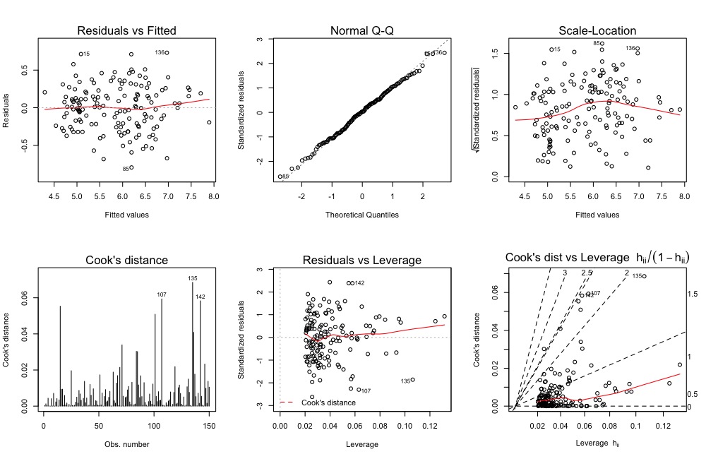
lm.object <- lm(Sepal.Length ~., data = iris)

The original visualization:

par(mfrow = c(2,3))
plot(lm.object, which = 1:6)

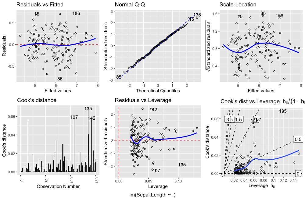
The updated visualization:

ggDiagnose(lm.object, which = 1:6)

ggDiagnose.lm allows for similar parameter inputs as plot.lm but also includes additional ones. This may changes as the package evolves.

`ggDiagnose.glmnet`

library(glmnet)
glmnet.object <- glmnet(y = iris$Sepal.Length, 
                           x = model.matrix(Sepal.Length~., data = iris))

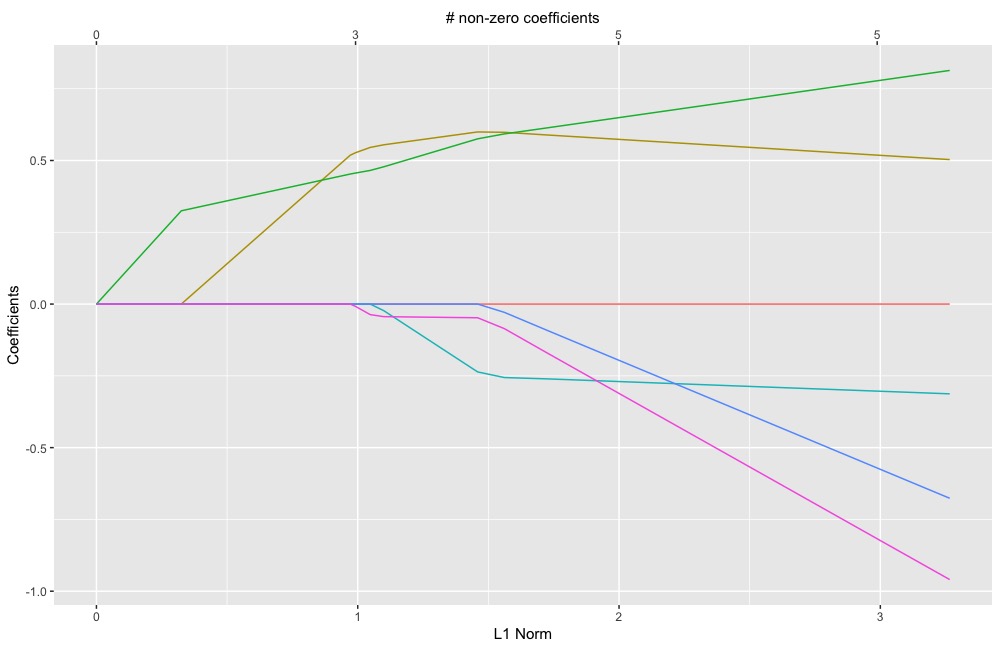
The original visualization:

plot(glmnet.object)

The updated visualization:

ggDiagnose(glmnet.object)

`ggDiagnose.cv.glmnet`

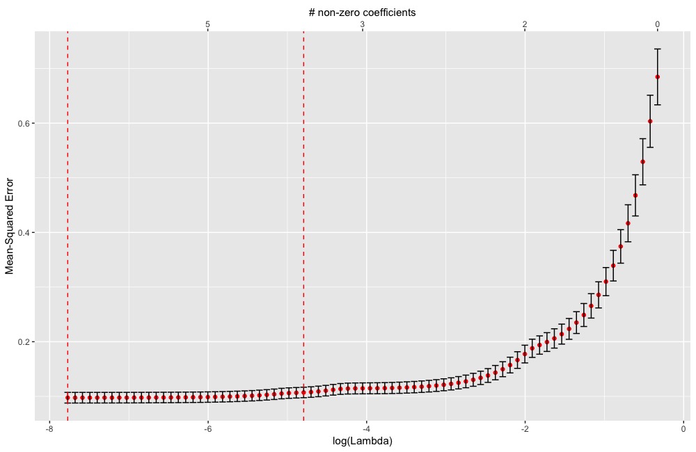
cv.glmnet.object <- cv.glmnet(y = iris$Sepal.Length, 
                              x = model.matrix(Sepal.Length~., data = iris))

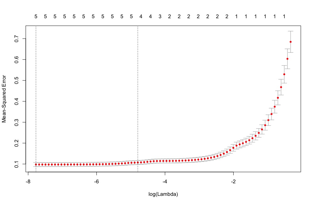
The original visualization:

plot(cv.glmnet.object)

The updated visualization:

ggDiagnose(cv.glmnet.object)

ggDiagnose.Gam

library(gam)
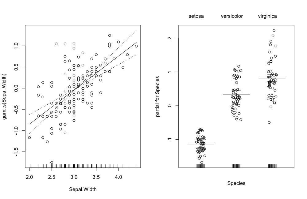
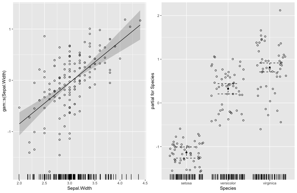
gam.object <- gam::gam(Sepal.Length ~ gam::s(Sepal.Width) + Species,
                  data = iris)

The original visualization:

par(mfrow = c(1,2))
plot(gam.object, se = TRUE, residuals = TRUE)

The updated visualization:

ggDiagnose(gam.object, residuals = TRUE) # se = TRUE by default

ggDiagnose.tree

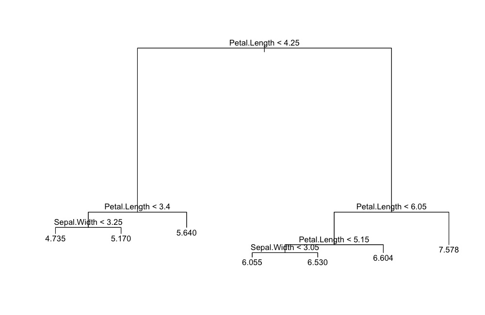
Note, for more perfect replication of the base plot function add + ggdendro::theme_dendro() which drops all ggplot background elements.

library(tree)

tree.object <- tree(Sepal.Length ~., data = iris)

The original visualization:

plot(tree.object)
text(tree.object)

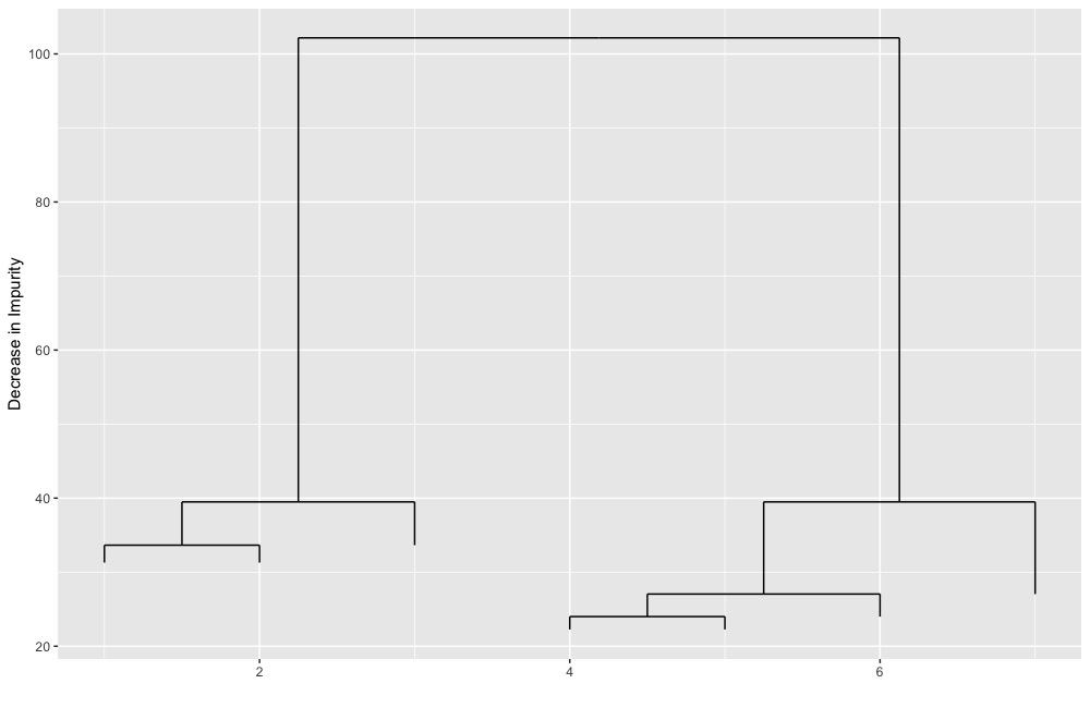
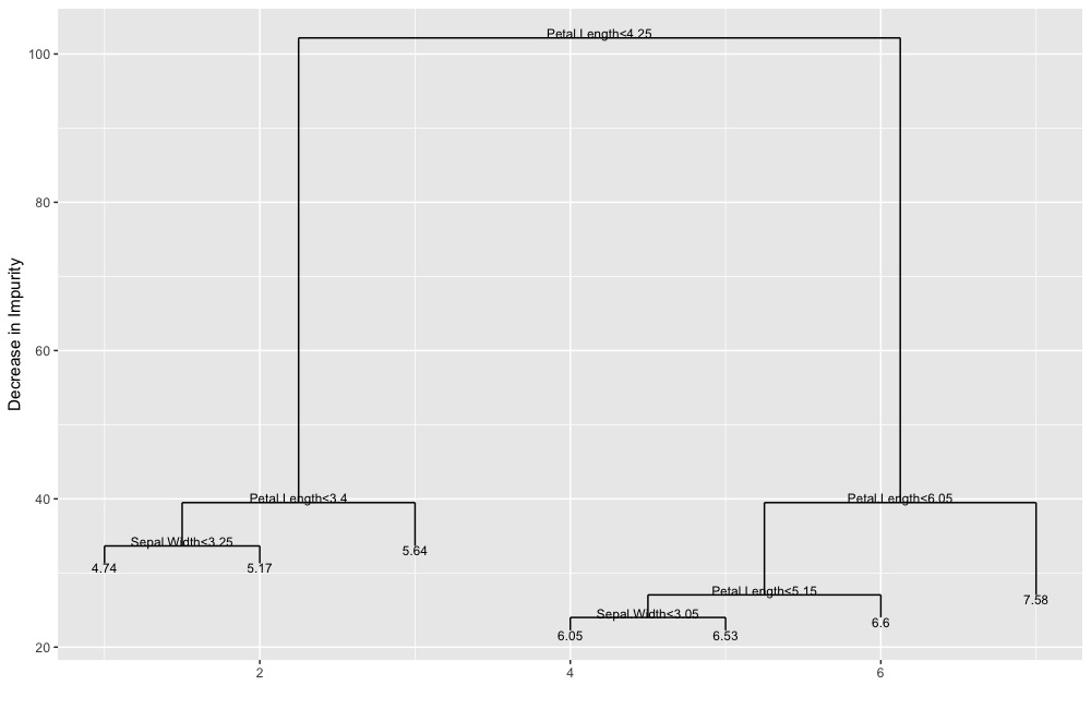
The updated visualization (followed by quick improvement):

ggDiagnose(tree.object, split.labels = FALSE)

ggDiagnose(tree.object, split.labels = TRUE,
           leaf.labels = TRUE)

ggDiagnose.matrix

ggDiagnose.matrix actually can create a visualization of a matrix similar to the "base R"'s image or heatmap.

Heatmap visualization

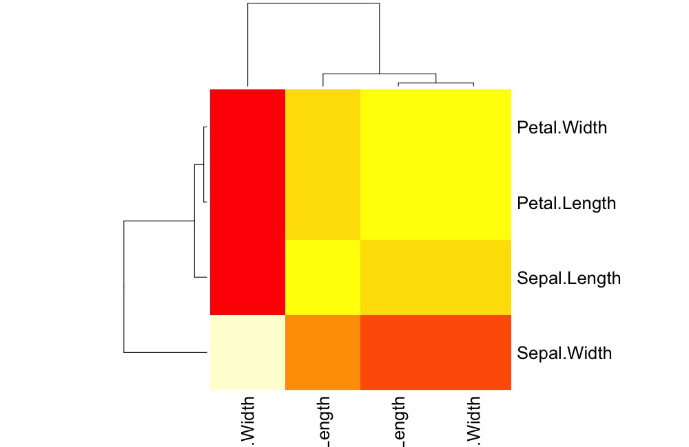
The original visualization using heatmap

data(iris)
iris_c <- iris %>% select(-Species) %>% cor %>% as.matrix 

heatmap(iris_c)

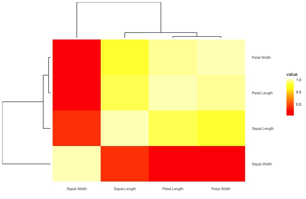
The updated visualization (note that we did a little manipulation to make the default color scheme match.) We may make this the default within the function later.

ggDiagnose.matrix(iris_c, type = "heatmap",return = T, show.plot = F)$ggout + 
  scale_fill_gradientn(colours = grDevices::heat.colors(10))

Image visualization

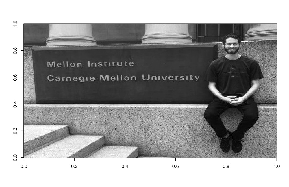
The original function image:

myurl = "http://stat.cmu.edu/~bpleroy/images/me.jpg"
data = jpeg::readJPEG(RCurl::getURLContent(myurl))[,,1]
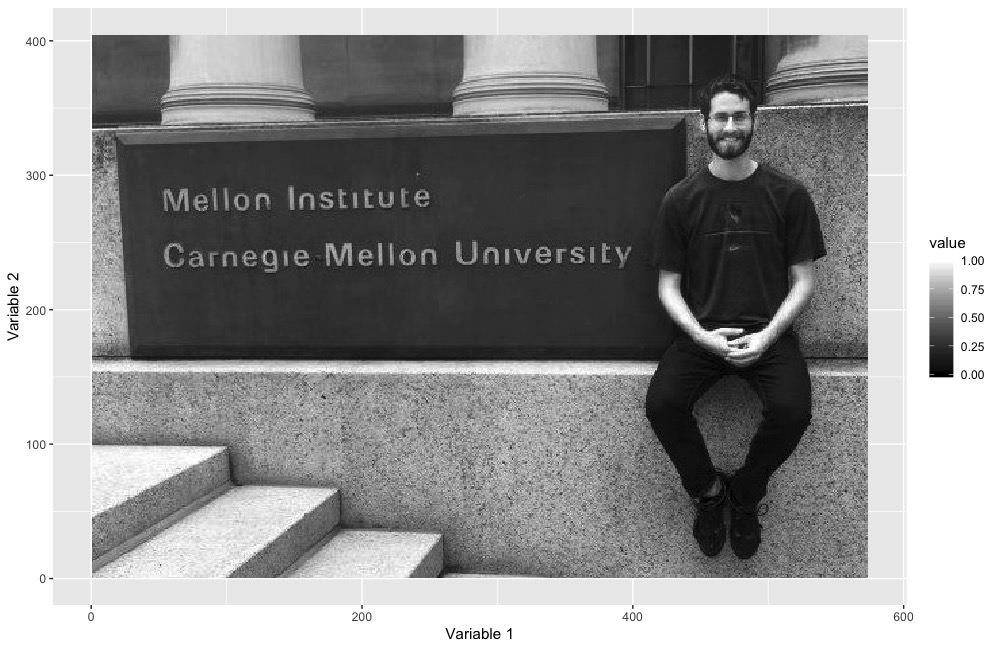
data = t(data)[,rev(1:nrow(data))]

image(data, col = grey(seq(0, 1, length = 256)))

The updated visualization (note that again we changed the base color to match with the expected output for this image.)

ggDiagnose.matrix(data, type = "image",return =T, show.plot=F)$ggout + 
  scale_fill_gradient(high = "white",low = "black")

`dfCompile`

`dfCompile.lm`

> library(dplyr)
> lm.object <- lm(Sepal.Length ~., data = iris)

> dfCompile(lm.object) %>% names
 [1] "Sepal.Length"          "Sepal.Width"           "Petal.Length"         
 [4] "Petal.Width"           "Species"               ".index"               
 [7] ".labels.id"            ".weights"              ".yhat"                
[10] ".resid"                ".leverage"             ".cooksd"              
[13] ".weighted.resid"       ".std.resid"            ".sqrt.abs.resid"      
[16] ".pearson.resid"        ".std.pearson.resid"    ".logit.leverage"      
[19] ".ordering.resid"       ".ordering.std.resid"   ".ordering.cooks"      
[22] ".non.extreme.leverage"

> dfCompile(lm.object) %>% head(2) # needs package dplyr for "%>%"
  Sepal.Length Sepal.Width Petal.Length Petal.Width Species .index .labels.id
1          5.1         3.5          1.4         0.2  setosa      1          1
2          4.9         3.0          1.4         0.2  setosa      2          2
  .weights    .yhat     .resid  .leverage      .cooksd .weighted.resid
1        1 5.004788 0.09521198 0.02131150 0.0003570856      0.09521198
2        1 4.756844 0.14315645 0.03230694 0.0012517183      0.14315645
  .std.resid .sqrt.abs.resid .pearson.resid .std.pearson.resid .logit.leverage
1  0.3136729       0.5600651     0.09521198          0.3136729      0.02177557
2  0.4742964       0.6886918     0.14315645          0.4742964      0.03338553
  .ordering.resid .ordering.std.resid .ordering.cooks .non.extreme.leverage
1             115                 115             124                  TRUE
2              98                  98              96                  TRUE

`dfCompile.glmnet`

> library(glmnet)
> glmnet.object <- glmnet(y = iris$Sepal.Length,
                 x = model.matrix(Sepal.Length~., data = iris))

> dfCompile(glmnet.object) %>% names # needs package dplyr for "%>%"
[1] ".log.lambda"      "variable"         "beta.value"       ".norm"           
[5] ".dev"             ".number.non.zero"

> dfCompile(glmnet.object) %>% head(2) # needs package dplyr for "%>%"
  .log.lambda     variable beta.value      .norm      .dev .number.non.zero
1  -0.3292550 X.Intercept.          0 0.00000000 0.0000000                0
2  -0.4222888 X.Intercept.          0 0.03632753 0.1290269                1

`dfCompile.cv.glmnet`

> library(glmnet)
> cv.glmnet.object <- cv.glmnet(y = iris$Sepal.Length,
                                x = model.matrix(Sepal.Length~., data = iris))

> dfCompile(cv.glmnet.object) %>% names # needs package dplyr for "%>%"
[1] "cross.validated.error"        "cross.validation.upper.error"
[3] "cross.validation.lower.error" "number.non.zero"             
[5] ".log.lambda"

> dfCompile(cv.glmnet.object) %>% head(2) # needs package dplyr for "%>%"
   cross.validated.error cross.validation.upper.error
s0             0.6840064                    0.7340895
s1             0.6009296                    0.6487392
   cross.validation.lower.error number.non.zero .log.lambda
s0                    0.6339234               0  -0.3292550
s1                    0.5531200               1  -0.4222888

`dfCompile.Gam`

> library(gam)
> gam.object <- gam::gam(Sepal.Length ~ gam::s(Sepal.Width) + Species,
                         data = iris)

> dfCompile(gam.object) %>% names # needs package dplyr for "%>%"
 [1] "Sepal.Length"                       
 [2] "Sepal.Width"                        
 [3] "Petal.Length"                       
 [4] "Petal.Width"                        
 [5] "Species"                            
 [6] ".resid"                             
 [7] ".smooth.gam.s.Sepal.Width."         
 [8] ".smooth.Species"                    
 [9] ".se.smooth.gam.s.Sepal.Width..upper"
[10] ".se.smooth.Species.upper"           
[11] ".se.smooth.gam.s.Sepal.Width..lower"
[12] ".se.smooth.Species.lower"

> dfCompile(gam.object) %>% head(2) # needs package dplyr for "%>%"
  Sepal.Length Sepal.Width Petal.Length Petal.Width Species     .resid
1          5.1         3.5          1.4         0.2  setosa 0.03614362
2          4.9         3.0          1.4         0.2  setosa 0.23792407
  .smooth.gam.s.Sepal.Width. .smooth.Species
1                 0.35570963       -1.135187
2                -0.04607082       -1.135187
  .se.smooth.gam.s.Sepal.Width..upper .se.smooth.Species.upper
1                          0.44985507                -1.006952
2                         -0.03387729                -1.006952
  .se.smooth.gam.s.Sepal.Width..lower .se.smooth.Species.lower
1                          0.26156418                -1.263422
2                         -0.05826436                -1.263422

`dfCompile.tree`

> library(gam)
> gam.object <- gam::gam(Sepal.Length ~ gam::s(Sepal.Width) + Species,
                         data = iris)

> dfCompile(tree.object) %>% length # needs package dplyr for "%>%"
[1] 4

> dfCompile(tree.object)$segments %>% head # needs package dplyr for "%>%"
     .x       .y .xend     .yend .n
2 2.250 39.49191 2.250 102.16833 73
3 1.500 33.64903 1.500  39.49191 53
4 1.000 31.29592 1.000  33.64903 20
5 2.000 31.29592 2.000  33.64903 33
6 3.000 33.64903 3.000  39.49191 20
7 6.125 39.49191 6.125 102.16833 77

> dfCompile(tree.object)$labels %>% head # needs package dplyr for "%>%"
      .x        .y            .label
1 4.1875 102.16833 Petal.Length<4.25
2 2.2500  39.49191  Petal.Length<3.4
3 1.5000  33.64903  Sepal.Width<3.25
4 6.1250  39.49191 Petal.Length<6.05
5 5.2500  27.04709 Petal.Length<5.15
6 4.5000  24.00201  Sepal.Width<3.05

> dfCompile(tree.object)$leaf_labels %>% head # needs package dplyr for "%>%"
   .x       .y .label    .yval
4   1 31.29592   4.74 4.735000
5   2 31.29592   5.17 5.169697
6   3 33.64903   5.64 5.640000
10  4 22.26715   6.05 6.054545
11  5 22.26715   6.53 6.530000
12  6 24.00201   6.60 6.604000

`dfCompile.matrix`

This function has an option type that takes either image or heatmap (see reference documentation).

Note that both also provide the potential for row and column associated dendrograms.

> dfCompile(iris_c, type = "heatmap")$df %>% head #needs package dplyr for "%>%"
         .var1        .var2      value
1  Sepal.Width  Sepal.Width  1.0000000
2 Sepal.Length  Sepal.Width -0.1175698
3 Petal.Length  Sepal.Width -0.4284401
4  Petal.Width  Sepal.Width -0.3661259
5  Sepal.Width Sepal.Length -0.1175698
6 Sepal.Length Sepal.Length  1.0000000

> dfCompile(iris_c, type = "image")$df %>% head
         .var1        .var2      value
1 Sepal.Length Sepal.Length  1.0000000
2  Sepal.Width Sepal.Length -0.1175698
3 Petal.Length Sepal.Length  0.8717538
4  Petal.Width Sepal.Length  0.8179411
5 Sepal.Length  Sepal.Width -0.1175698
6  Sepal.Width  Sepal.Width  1.0000000

TODO:

Overarching (when making new object functionality):

1. check what broom does for each object. Document when broom doesn't create what we need for the visualizations.

ggDiagnose (models):

1. lm, glm (from stats package): ggDiagnose.lm
2. Gam (from the original gam package - not mgcv - or at least not first round)
3. glmnet (from glmnet packages): ggDiagnose.glmnet, ggDiagnose.cv.glmnet
- plot.mrelnet, plot.multnet needed?
4. tree (from tree package - could also one from rpart package - use ggdendro and see examples from ggdendro.
5. randomForest
6. mclust (multiple objects - multiple options for Mclust graphic. - will take time)
7. PCA/factor analysis, etc objects

CM 36-402 models' from Cosma's book

8. npreg from np, kernel regression (pg 124)
- looks like a 3d option (plotly?) and a partial-dependence like plot
9. tree stuff - plot slices 2d? (pg ~300)

ggVis (other objects):

1. sp
2. dendrogram (very similar to tree, and there is already a ggdendro... package that would do it better. Let's not do this for now)
3. matrix (for heatmap? or image?) - let's do both for now.

packages that I'm not sure can be done:

1. lme4 (these objects don't seem to have plot._ functions to emulate.)
2. kde2d - from MASS (actually just produces a list ...) - but z could be dealt with a matrix that you want to do "image" to.
9. ranger (better RF package?) (doesn't actually have plot function for ranger objects...)

teaching:

1. In examples for each function provide code to create some / all of the plots in a more basic manner with straight use of tidyverse. (Is this worthwhile? maybe for non-trivial/non standard ggplot2 graphics?)

best coding practices:

1. decide which parameters are passed to the visualization functions and how they differ / are the same of the plot implementation. For all visuals we have show.plot and return parameters.

documentation:

1. create a new file for package documentation. See: http://r-pkgs.had.co.nz/man.html#man-packages

things to look into:

S3 methods? - should the whole thing be a S3 method?

Write a blog post about putting a changing axis on top, link to the one where they transform the equation. Mention Hadley's thoughts on the matter.

ideas for tests:

for all check the data frame coming out of ggDiagnose vs dfCompile,
look at the names of the data frame returned by dfCompile
check return options for ggDiagnose

readme needs:

Probably should be showcasing dfCompile as well... how to do so in .md...