tidypaleo

Working with multi-proxy paleo-archive data is inherently difficult. There are multiple locations, multiple parameters, and a lot of discipline-specific norms for plot layout and notation. This package simplifies a few workflows to promote the use of R and reproducible documents in paleo-based studies.

Installation

You can install tidypaleo from github with:

# install.packages("devtools")
devtools::install_github("paleolimbot/tidypaleo")

To get the most out of strat diagrams, you will also need the patchwork package by [@thomasp85]((https://github.com/thomasp85). You can also install this from GitHub:

# install.packages("devtools")
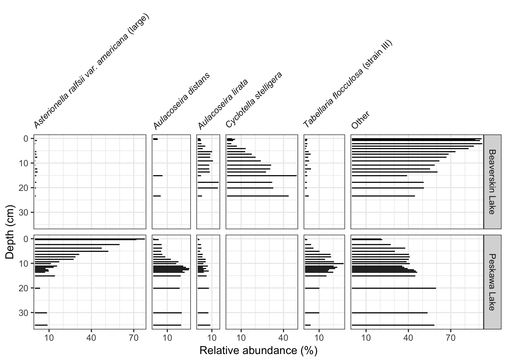
devtools::install_github("thomasp85/patchwork")

Examples

Age-depth models

Stratigraphic diagrams

This package exposes a number of functions useful when creating stratigraphic diatrams, including facet_abundanceh(), which combines several other functions to help create stratigraphic plots using ggplot2. The geom_col_segsh() geometry draws horizontal sements, which are commonly used to show species abundance data.

library(ggplot2)
library(tidypaleo)
theme_set(theme_bw())

ggplot(keji_lakes_plottable, aes(x = rel_abund, y = depth)) +
  geom_col_segsh() +
  scale_y_reverse() +
  facet_abundanceh(vars(taxon), grouping = vars(location)) +
  labs(y = "Depth (cm)")

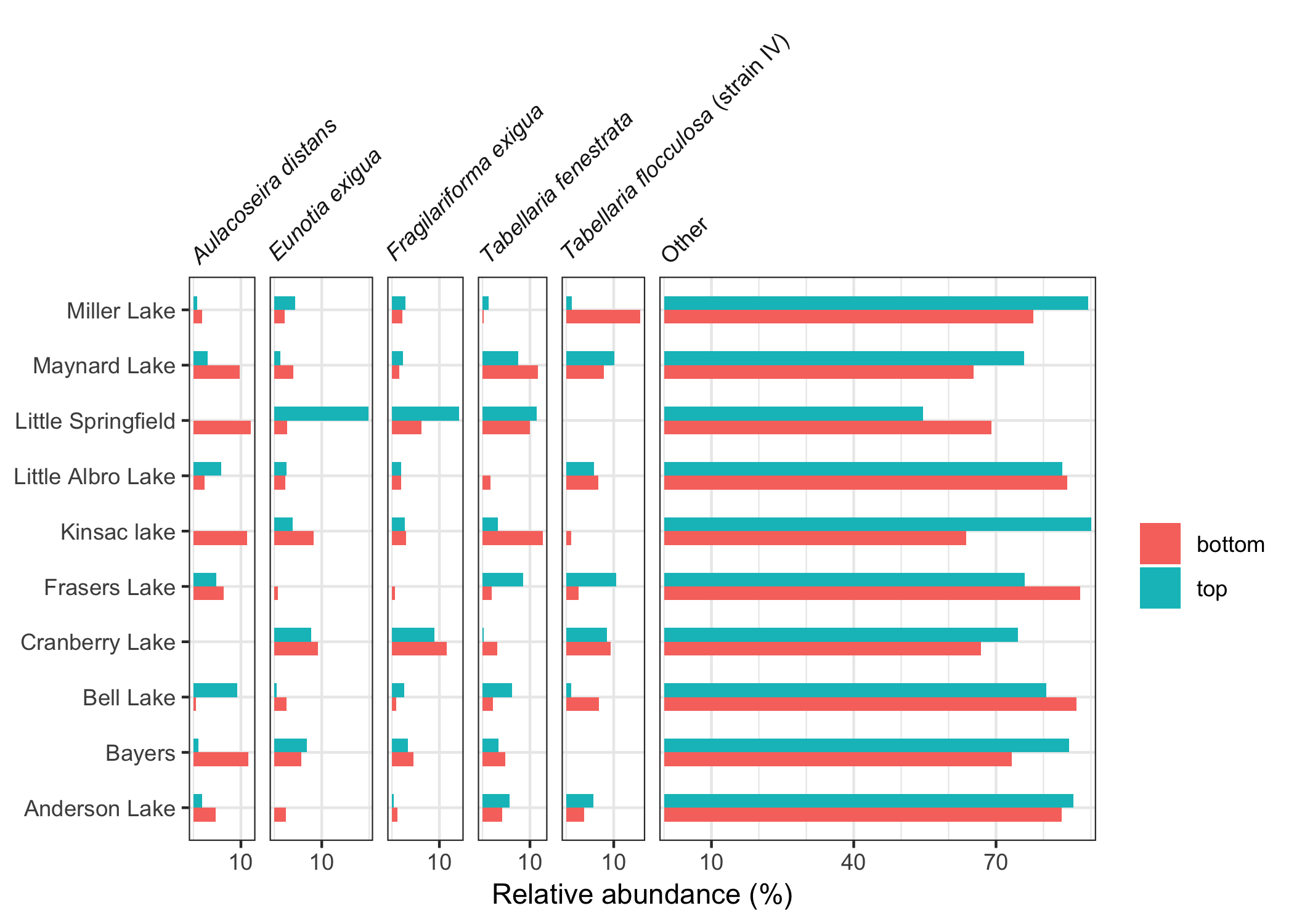
Relative abundance data with a discrete y axis can be drawn using geom_colh() and position_dodgev() from the ggstance package.

ggplot(halifax_lakes_plottable, aes(x = rel_abund, y = location, fill = sample_type)) +
  geom_colh(width = 0.5, position = "dodgev") +
  facet_abundanceh(vars(taxon)) +
  labs(fill = NULL, y = NULL)

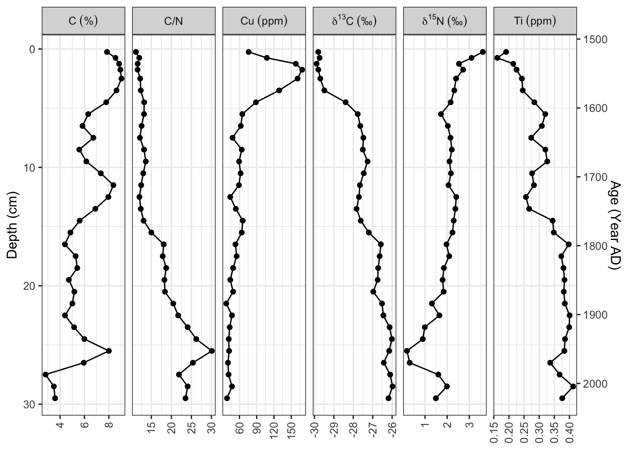
Age depth models can be constructed (using age_depth_model()) and used to draw second axes on stratigraphic plots (using scale_y_depth_age()). The facet_geochem() function wraps facet_wrap(), and includes a labeller (label_geochem) that can add units, and automatically renames d15N, d13C and d18O such that they are labelled correctly.

alta_adm <- age_depth_model(
  alta_lake_bacon_ages, 
  depth = depth_cm,
  age = 1950 - age_weighted_mean_year_BP
)

ggplot(alta_lake_geochem, aes(x = value, y = depth)) +
  geom_lineh() +
  geom_point() +
  scale_y_depth_age(alta_adm, age_name = "Age (Year AD)") +
  facet_geochem_wraph(
    vars(param), 
    nrow = 1, 
    units = c(
      C = "%",
      Cu = "ppm",
      Ti = "ppm",
      d15N = "‰",
      d13C = "‰"
    )
  ) +
  labs(y = "Depth (cm)", x = NULL)

benmarwick/tidypaleo

tidypaleo

Installation

Examples

Age-depth models

Stratigraphic diagrams