| NN ODEsolver: | Code that numerically solves ODEs using Neural Networks in an unsupervised manner |
| Authors: | Liam L.H. Lau, Denis Werth |
| Version: | 1.0 |
| Homepage: | https://github.com/deniswerth/NeuralNetwork_ODEsolver |
Feedforward neural networks are able to approximate any continuous function at any level of accuracy. This is a loose statement of the Universal Approximation Theorem for neural networks. Although there is open source code for neural network solvers for ODEs and PDEs, the difference is that this network trains to fit the differential equation and boundary/ initial conditions at the same time. We also suggest that the loss is approximately the mean absolute error, without the need of having the true solution.
The paper can be found here: https://arxiv.org/abs/2005.14090
All examples from the paper can be reproduced with the code provided, a walk through is provided in the examples section below.
- To replicate the plots in the paper and in Examples below, comment out all the
if __name__ == "__main__":sections except the particular example you want to keep.
Imported in __Main__.py by:
from ODEsolver import ODEsolverInitialization of the class is executed in __Main__.py like so:
ODEsolver(order, diffeq, x, initial_condition, epochs, architecture, initializer, activation, optimizer, prediction_save, weights_save)| Argument | Description | Example |
|---|---|---|
| Order: int | Order of the differential equation | 2 |
| diffeq: string | Differential equation name | "schrodinger" |
| x: ndarray | Sampled domain | np.linspace(-5, 5, 100) |
| initial_condition: tuple | Initial condition for the differential equation | ((x0, y0), (dx0, dy0)) |
| epochs: int | The number of epochs the neural net is trained for | 10000 |
| architecture: list | Architecture of the densely connected hidden layers | [30, 30, 30] |
| initializer: string | Initializer of the neural network parameters | "GlorotNormal" |
| activation: string | Activation function used for the hidden layers | "sigmoid" |
| optimizer: string | optimizer used for gradient descent | "Adam" |
| prediction_save: bool | Toggle for whether the prediction at each epoch is saved. Used for animation | True/False |
| weights_save: bool | Toggle for whether the weights and biases at each epoch are saved. Can be used for trajectory plots on the loss surface | True/False |
Imported in __Main__.py by:
from Dictionary import Dictionary
D = Dictionary()
Dict = D.Dict- Dictionary class that contains the initializers, activation functions and optimizers that
Imported in __Main__.py by:
from DiffEq import DiffEq- Differential equation class that contains definition of differential equation problem. Three examples are given: a first order ODE; nth stationary Schrodinger equation with a harmonic potential and a burst equation.
A custom differential equation can be defined as the following in
DiffEq.py:
if self.diffeq == "name":
    # x should be written as self.x; y should be written as self.y; dy/dx should be written as self.dydx and d2y/dx2 should be written as self.d2ydx2
self.eq = self.d2ydx2 + self.dydx + self.y - tf.math.exp(-self.x) # Your custom differential equation- Currently, the code only supports up to second order. However higher order derivatives can be implemented by editing the
y_gradientsfunction for the Neural Network Solver class inODEsolver.py. For example, third order can be accessed by using the following code snippet:
def y_gradients(self, x):
    """
    Computes the gradient of y.
    """
    with tf.GradientTape() as tape1:
        tape1.watch(x)
        with tf.GradientTape() as tape2:
            tape2.watch(x)
            with tf.GradientTape() as tape3:
                tape3.watch(x)
                y = self.NN_output(x)
            dy_dx = tape3.gradient(y, x)
        d2y_dx2 = tape2.gradient(dy_dx,x)
    d3y_dx3 = tape1.gradient(d2y_dx2,x)
    return y, dy_dx, d2y_dx2, d3y_dx3
Make sure to edit the differential_cost function for the Neural Network Solver class in ODEsolver.py to include the extra derivatives:
y, dydx, d2ydx2, d3ydx3 = self.y_gradients(x)de = DiffEq(self.diffeq, x, y, dydx, d2ydx2, d3ydx3)Also make sure to also edit the custom_cost function in ODEsolver.py to include extra boundary terms, an example is given for a third order derivative:
if self.order == 3:
    x0 = np.float64(self.initial_condition[0][0])
    y0 = np.float64(self.initial_condition[0][1])
    dx0 = np.float64(self.initial_condition[1][0])
    dy0 = np.float64(self.initial_condition[1][1])
    d2x0 = np.float64(self.initial_condition[2][0])
    d2y0 = np.float64(self.initial_condition[2][1])
    def loss(y_true, y_pred):
        differential_cost_term = tf.math.reduce_sum(self.differential_cost(x))
        boundary_cost_term = tf.square(self.NN_output(np.asarray([[x0]]))[0][0] - y0)
        boundary_cost_term += tf.square(self.NN_output(np.asarray([[dx0]]))[0][0] - dy0)
        boundary_cost_term += tf.square(self.NN_output(np.asarray([[d2x0]]))[0][0] - d2y0)
        return differential_cost_term/self.n + boundary_cost_term
    return loss
The third order derivative will now be available in DiffEq.py using self.d3ydx3
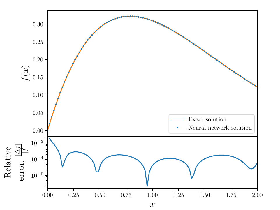
- Using the following differential equation and a boundary condition y = 0 at x = 0:
- Neural Network Solver numerical solution is overlayed on the true solution. Note the solution is effectively continuous in the domain
- A speed up animation of the training process:
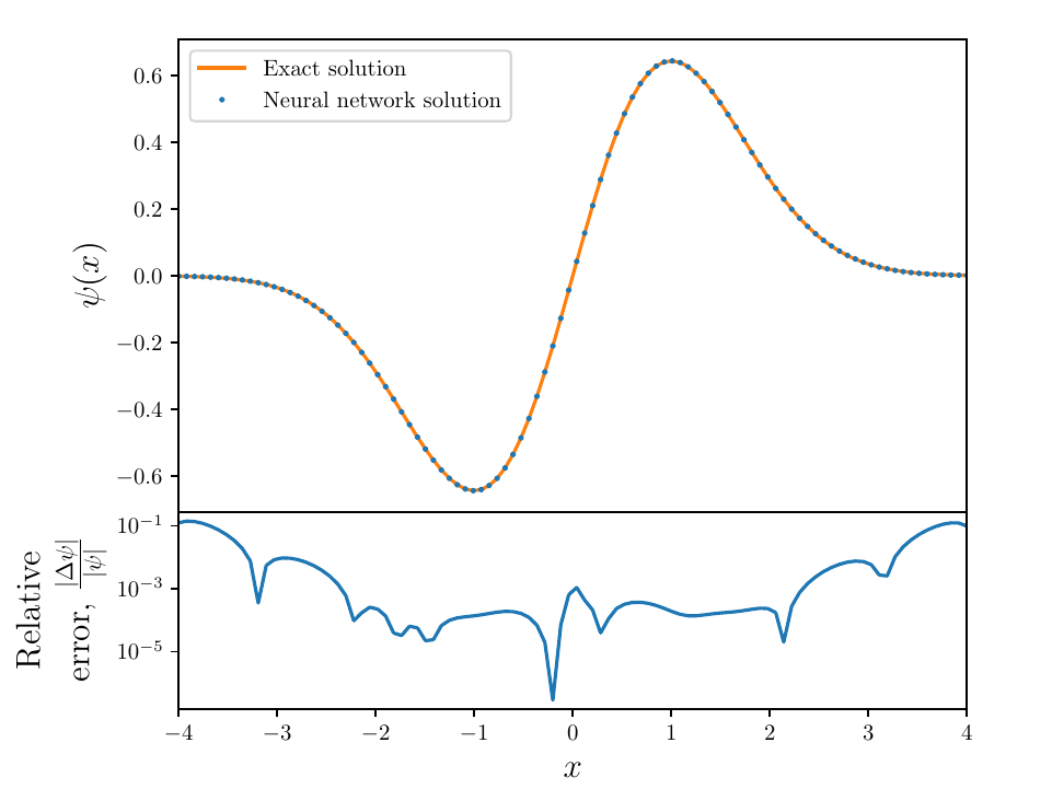
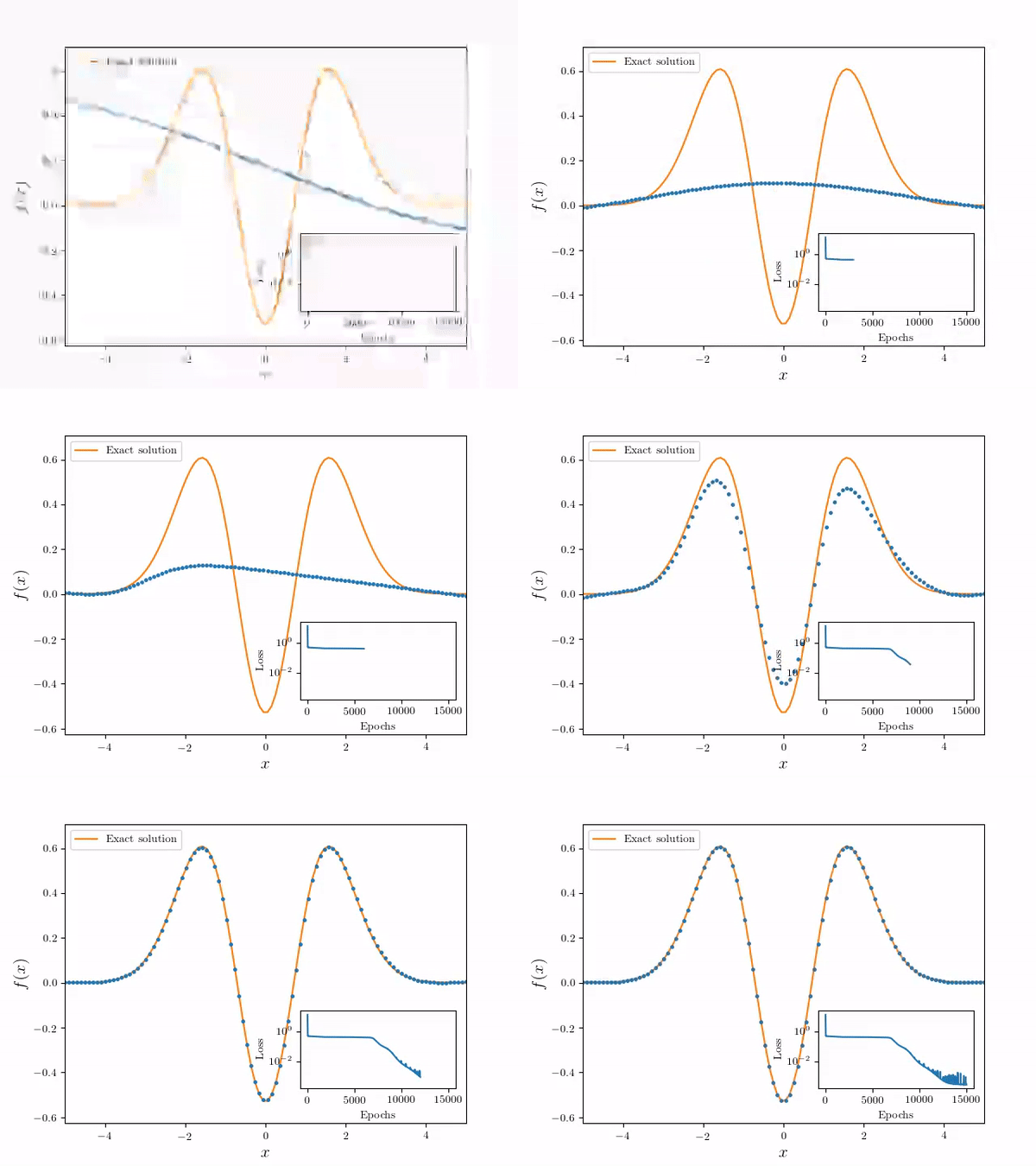
- Using the following differential equation and Dirichlet boundary conditions:
- Neural Network Solver numerical solution is overlayed on the true solution. Note the solution is effectively continuous in the domain
- A speed up animation of the training process:
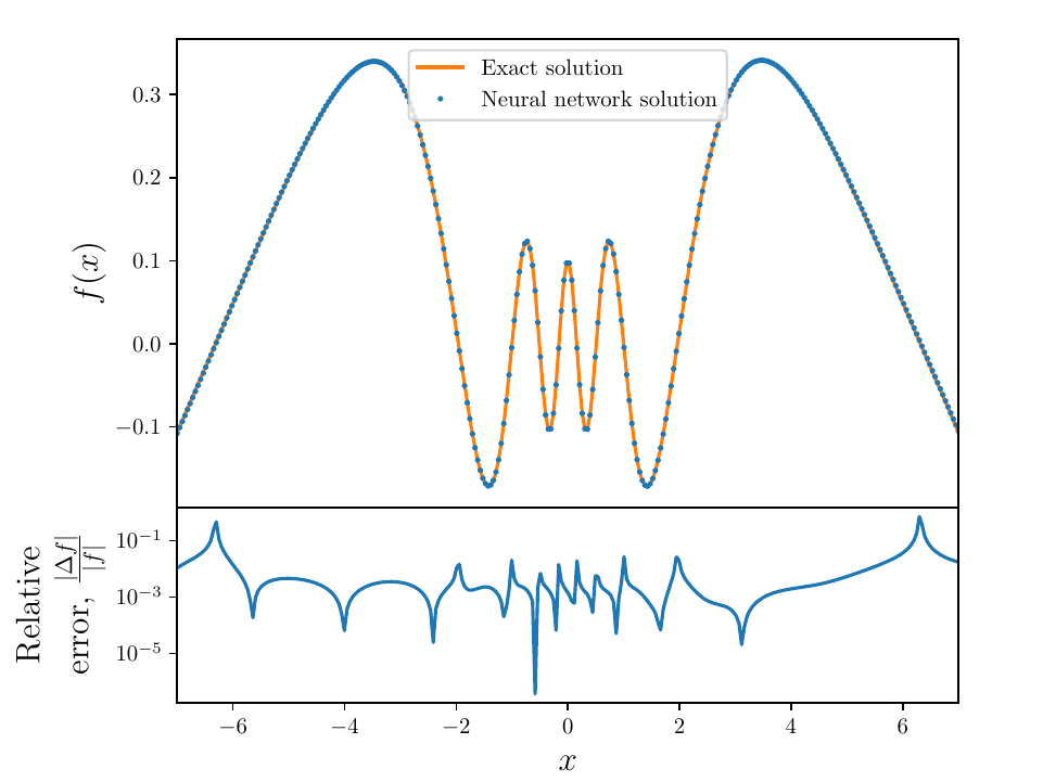
- Using the following differential equation and Dirichlet boundary conditions:
- Neural Network Solver numerical solution is overlayed on the true solution. Note the solution is effectively continuous in the domain
- A speed up animation of the training process:


