Berthy T. Feng, Alexander C. Ogren, Chiara Daraio, Katherine L. Bouman. "Visual Vibration Tomography: Estimating Interior Material Properties from Monocular Video." In Proceedings of the IEEE/CVF Conference on Computer Vision and Pattern Recognition (CVPR), 2022 (Oral).
The codebase is written in Python and doesn't require many special packages, except the Python wrapper for FEniCS known as DOLFIN.
$ conda update conda
$ conda create -n vvt python=3.7
$ conda activate vvt
$ conda config --add channels conda-forge
$ conda config --add channels anaconda
Note that Conda's environment solving step could take a while.
$ conda install --file requirements.txt
$ pip install pyrtools
The notebook demo1_simulated_cube.ipynb walks through end-to-end estimation
from an input video. Please download simulated cube data and place them in the simulated_data folder. The demo specifically works with defect03.
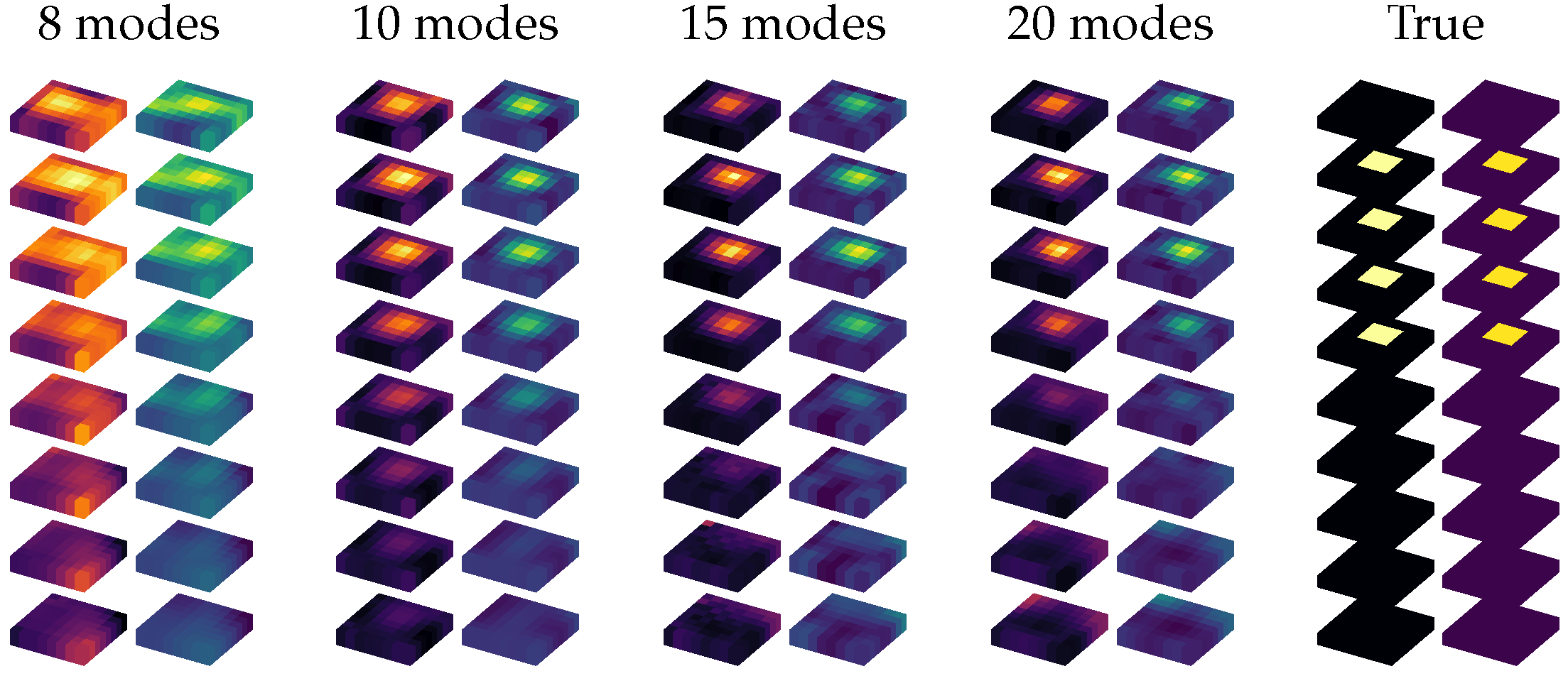
(Paper Fig. 4) Reconstruction of "defect03" as number of input modes increases.
A damped cube typically requires modal observations from multiple videos. As such, we split the process into two notebooks:
demo2.1_real_cube_mode_extraction.ipynbwalks through motion and image-space mode extraction from one video. The notebook can be repeatedly run for multiple videos of the same object, saving modal observations from each one.demo2.2_real_cube_inference.ipynbtakes the modal observations from multiple videos and averages them to solve for material properties.
Please download the real Jello cube data and place them in the real_data folder. Modal observations from all three videos are already provided, so you can skip step (1).
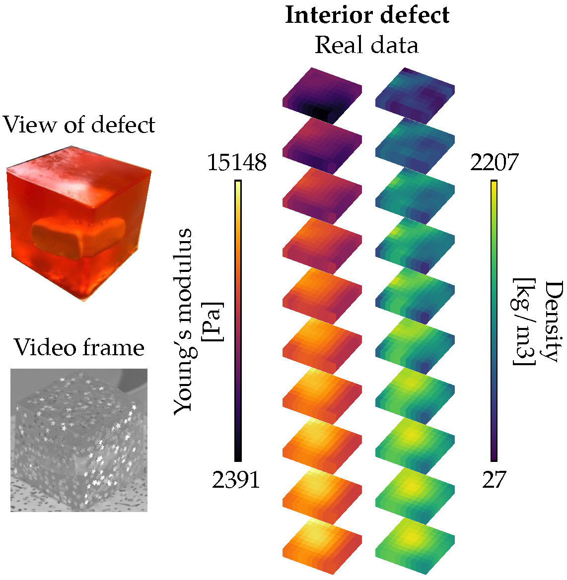
(Paper Fig. 11) Reconstructed material properties of a real Jello cube.
The simulated dataset
contains 12 different defect cubes. defect01-defect12
are the undamped versions, and damped_defect01-damped_defect12 are the damped
versions. Additionally, defect_center is an undamped cube with a perfectly-centered
defect.
The data for each object is stored in a folder (e.g., simulated_data/defect01)
that contains the following files:
true_stiffness.npy,true_density.npy: The true material properties used in the forward model. The forward model is a 10x10x10 hexahedral mesh, so each file is a 1D NumPy array containing the voxel-wise material-property values.{initial_condition}/transient.mat: The COMSOL transient analysis results for a particular initial condition. This file is used to create the animated video,{initial_condition}/transient.gif. Since the undamped cubes have sufficient modal expression from one initial condition, only thetop_front_plucktransient analysis results are included. The damped cubes may need modal information from multiple videos, so the transient analysis results of 5 initial conditions are provided:top_front_pluck,top_back_pluck,top_right_pluck,top_left_pluck,top_right_twist.modal.mat: The COMSOL modal analysis results. This file is not used in material-property estimation, but can be used to check the true full-field modes of the object.
An animated video takes up a lot of storage (~1.2 GB), so we provide a
limited number of pre-written videos, specifically for: defect_03, defect_08, and damped_defect_03.
For reference, we provide some files useful for making your own simulated cube data.
comsol/template.mph is the COMSOL file that can be edited to make your
own cube forward model. For example, you can change the dimensions of the box,
defect shape and location, and material properties.
comsol/run_comsol_sim.m takes the COMSOL file, run transient analyses
and a modal analysis, and saves the results of these analyses.
To make an animated video from COMSOL transient analysis results, run
$ python make_comsol_animation.py {OBJ_NAME} {SIM_NAME}
where OBJ_NAME is the cube sample (e.g., "defect_01"), and SIM_NAME is the transient-analysis name (e.g., "top_front_pluck"). The script writes a GIF named transient.gif in the same folder that contains the transient.mat file. To speed up motion extraction, you can crop the GIF frames tightly to the cube.
The easiest results to reproduce with this repo are reconstructions for simulated_data/defect_03 and real_data/jello_cube. The paper includes figures for additional cases, including damped cubes and simulated/real drums.
The best way to work with damped cubes (e.g., simulated_data/damped_defect01) is to follow the process for the real Jello cube, i.e., with demo2.1_real_cube_mode_extraction.ipynb and demo2.2_real_cube_inference.ipynb. The video names and FPS will have to be specified accordingly, and the modal observations require some amount of qualitative hand-selection.
For clarity, we only provide code for working with cubes. Please contact bfeng@caltech.edu if you would like code for working with drums or other geometries.

