modelviz

Overview

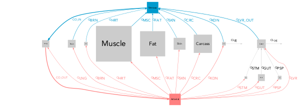
Automated generation of quantitative model diagrams for NONMEM.

Rationale

To facilitate model communication and evaluation through intuitive visual representation of their structure, parameter estimates, uncertainty (RSE) and variability (IIV).

Standard model diagrams

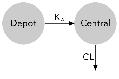
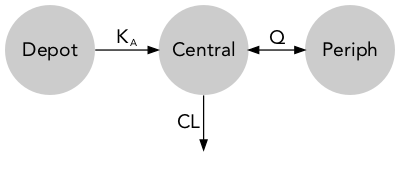
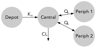
Models are commonly represented as standard model diagrams (SMD) showing their structural properties but lacking any information on parameter and must therefore be used along with a parameter table.

Quantitative model diagrams

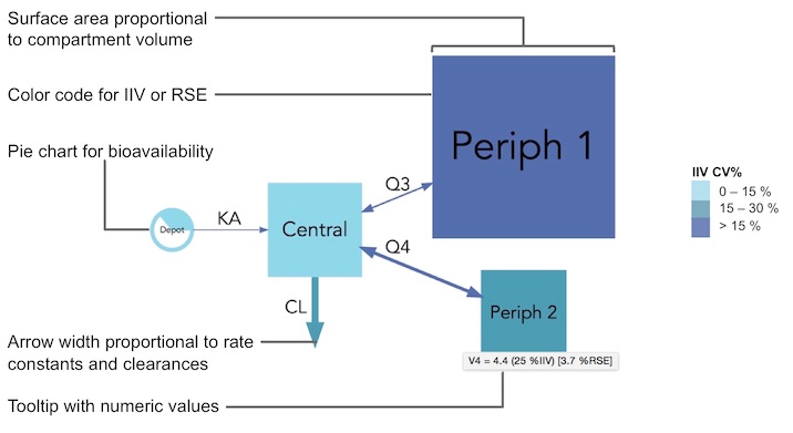
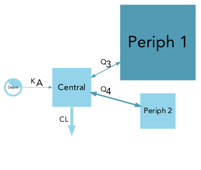
Quantitative model diagrams (QMD) are used to intuitively displays the structural model along with the parameter values and their uncertainty or variability.

Dynamic QMD

Dynamic QMD (dQMD) visually represent the dynamic processes proper to pharmacometric models. It allows to intuitively conceptualize complex processes such as feedback, non-linearity over time. dQMDs are currently only a concept and not a built-in feature of modelviz but will hopefully be coming in future updates.

`modelviz` installation

# Install modelviz package (first time only)
devtools::install_github("bguiastr/modelviz")

# Load the modelviz package
library(modelviz)

Workflow

Import dataset from a NONMEM run

qmd_info <- import_qmd_info(dir = '/nonmem/runs', runno = '101')

Generate QMD graph

qmd(qmd_info)

The `qmd_info` object

Structure

The qmd_info objects are lists of 8 levels:

descr : model description [character string, optional]
theta : theta typical values and RSE (%) [data.frame, optional]
omega : typical values (%) and RSE (%) [data.frame, optional]
data : individual parameter values [data.frame, optional]
advan : NONMEM ADVAN subroutine [integer, required]
des : NONMEM $DES subroutine [character strings, optional]
parsed_comp : parsed compartment information [data.frame, required]
parsed_arrow : parsed arrow information [data.frame, required]

Example of qmd_info for examples$onecomp

$descr
[1] "Example 1-comp: Nevirapine in HIV- and TB-infected south african (day values w/o rifampicin)"

$theta
         KA   CL     V
tvprm  3.57 2.76 137.0
rse   61.00 5.70   7.2

$omega
           KA       CL
tvprm 84.2615 55.40758
rse    0.8500  0.27000

$data
NULL

$advan
[1] 2

$des
NULL

$parsed_comp
    label  prm output
1   Depot <NA>  FALSE
2 Central    V   TRUE

$parsed_arrow
  from to prm     dir
1    1  2  KA forward
2    2 NA  CL forward

Creation of the `qmd_info` object

You can automatically create qmd_info via the function import_qmd_info() or manually with the help of the function skeleton_qmd_info().

The function import_qmd_info() read NONMEM model files (.mod or .lst type) and extract their key information:

$PROBLEM and file name will be stored in the descr
$SUBROUTINE will be stored in advan
The levels theta and omega are generated by associating parameter labels (read in the comments of $THETA and $OMEGA) to the final parameter values and RSE (read from the .ext file).
When available a parameter table (patab) will be stored in data [currently not used]
If ADVAN refers to a predefined NONMEM library (ADVAN 1-4,11-12) parsed_comp and parsed_arrow levels will be added to the qmd_info. If ADVAN refers to a differential equation system (ADVAN 6,8,13), the $MODEL and $DES block will be parsed to generate parsed_comp and parsed_arrow.

Differential equations parsing

The differential equation parser in modelviz works with most general ODE. The parser can handle terms in the form ±K*A(1), ±(CL/V)*A(1). In the first case K will be used to scale the arrow between A(1) and another compartment, in the second case CL will be used to scale the arrow between A(1) and V to scale the compartment A(1).

Differential equations should be written in their developed form. For example do not use -((CL+Q)/VC)*A(x) but rather -(CL/V)*A(x) -(Q/V)*A(x).

Other forms of equation starting by ± and containing a compartment amount e.g +(EMAX*A(1))/(EC50 + A(1)) will be properly parsed (arrows and compartment will be created) but no parameter will be used for scaling.

Advanced options

Scaling options

Model parameter can have extreme values and use different units (e.g volumes in mL or L), therefore the choice of the scaling function applied to compartment and arrows is open to the user. By default the compartment surface area is scaled proportionally to the volumes (comp_scale_fun = function(x) { sqrt(x) }) and arrows are scaled linearly to their rate or clearance (arrow_scale_fun = function(x) { x }). By customizing the comp_scale_fun and arrow_scale_fun constant (eg. 3), linear (eg. 2*x + 1), non-linear (eg. sqrt(x)), or complex (eg. logit transform) scaling functions can be applied.

Manual layout

Layout are automatically created by modelviz by minimizing the size of the graph and the arrows length. If as specific layout is desired the options rank can be used to order the compartments. The rank option can be used along with flipped. By default ranks are attributed from left to right, if flipped = TRUE ranks will be attributed from top to bottom.

Color scale

Color scales can be used to represent either IIV or RSE, which can be selected with the argument color_scaling = "RSE". A three-level color code will be defined, by default cutoff values are set at 25 % and 50 % but can be changed with the color_cutoff = c(25, 50) argument.

If no color scheme should be applied color_scaling can be set to NONE. The unscaled default grey color can be changed via unscaled_color.

To manually assign colors, the arguments arrow_color_manual and comp_color_manual can be used to define a color for each arrow and each compartment. Note the order of the arrows and compartment is following their order in the parsed_comp and parsed_arrow levels of the qmd_info object.

Visual aspect settings

Many other visual aspects of the diagrams can be changed such as the labels font (font = "Arial"), labels size (comp_fontsize = 1.5, arrow_fontsize = 1), disabling (labels = FALSE) or parsing (parse_labels = TRUE) arrow labels. The compartment filling can be disabled (filled = FALSE) nodes will then be represented by their edges only, the shape can also be changed for either scaled (scaled_shape = "square") or (unscaled_shape = "circle") compartments, and finally color transparency can be applied (alpha = 0.5).

PBPK options

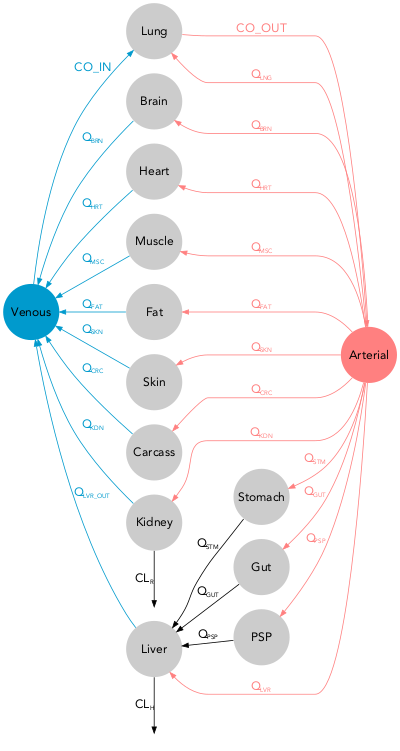
With PBPK models the options pbpk_layout = TRUE and color_scaling = "PBPK" must be used to obtain the classical layout with blue veins on one side and red arteries on the other. In order for modelviz to recognize the venous and arterial compartments, their exact label must be defined their label when they do not match the defaults (vein_comp_label = "venous", artery_comp_label = "arterial").

Additional options

Many more options can be used to change the aspect of the diagram via the graph_attrs argument. The graph_attrs argument must be provided as a data.frame and contain the attr, value and type columns e.g. data.frame(attr = "layout", value = "dot", type = "graph").

A few useful options are - splines [attr], ortho [value], graph [type] for square angled arrows, true [value] being the default value - rankdir [attr], 1 [value], graph [type] changes the space between compartments of a same rank - nodesep [attr], 1 [value], graph [type] changes the space between compartments of different rank

More options can be found here

Examples

The modelviz package contains 6 built-in examples intended to demonstrate the utility of QMD in various case scenarios and to familiarize users with the package.

One-compartment model

The example dataset onecomp contains typical pharmacokinetic parameters values and uncertainty for nevirapine. (Elsherbiny et al. 2009)

SMD

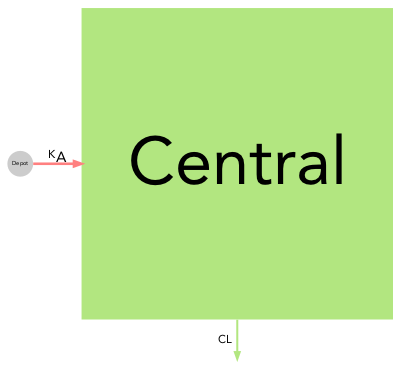
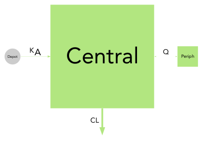
qmd(examples$onecomp, scaling = FALSE)

QMD

qmd(examples$onecomp, color_scaling = 'RSE')

Two-compartment model

The example dataset twocomp contains typical pharmacokinetic parameters values and uncertainty for miltefosine. (Dorlo et al. 2008)

SMD

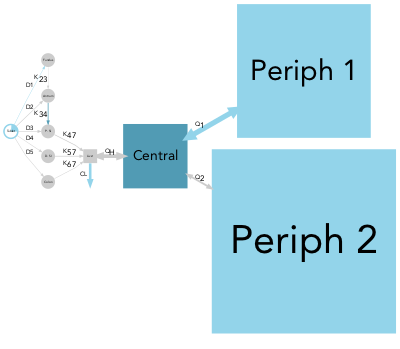
qmd(examples$twocomp, scaling = FALSE)

QMD

qmd(examples$twocomp, color_scaling = 'RSE')

Three-compartment model

The example dataset threecomp contains typical pharmacokinetic parameters values and uncertainty for ciclosporin in paediatric renal transplant candidates. (Fanta et al. 2007)

SMD

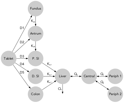
qmd(examples$threecomp, scaling = FALSE)

QMD

qmd(examples$threecomp, color_scaling = 'IIV')

Gastro-Intestinal Tansit Time (GITT) model

The example dataset gitt contains typical pharmacokinetic parameters values and uncertainty for felodipine gastro-intestinal transit time. (Hénin et al. 2012)

SMD

qmd(examples$gitt, scaling = FALSE,
    rank = c(1, 2, 2, 2, 2, 2, 3, 4, 5, 5))

QMD

qmd(examples$gitt, color_scaling = 'IIV',
    rank = c(1, 2, 2, 2, 2, 2, 3, 4, 5, 5),
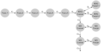
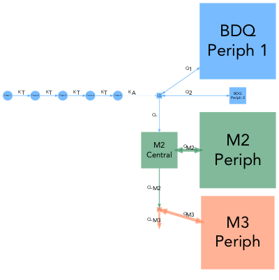
    arrow_scale_fun = function(x){sqrt(x)})

Bedaquiline metabolites model

The example dataset metabolite contains typical pharmacokinetic parameters values and uncertainty for bedaquiline and two of its metabolites. (Svensson et al. 2013)

SMD

qmd(examples$metabolite, scaling = FALSE,
    rank = c(1, 2, 3, 4, 5, 6, 7, 7, 6, 7, 6, 7))

QMD

qmd(examples$metabolite, color_scaling = 'IIV',
    rank = c(1, 2, 3, 4, 5, 6, 7, 7, 6, 7, 6, 7),
    comp_scale_fun = function(x){sqrt(x/50)},
    arrow_scale_fun = function(x){sqrt(x)},
    alpha = 0.6,
    comp_color_manual = c(rep('dodgerblue', 8), 
                          rep('seagreen', 2), 
                          rep('coral', 2)),
    arrow_color_manual = c(rep('dodgerblue', 8), 
                           rep('seagreen', 2), 
                           rep('coral', 2)))

Note: In this case manual color scheme has been applied

PBPK model

The example dataset pbpk contains typical pharmacokinetic parameters values for theophylline in adult male. (Björkman et al. 2004)

SMD

qmd(examples$pbpk, scaling = FALSE, 
    pbpk_layout = TRUE, color_scaling = 'PBPK')

QMD

qmd(examples$pbpk, flipped = TRUE
    pbpk_layout = TRUE, color_scaling = 'PBPK',
    arrow_scale_fun = function(x){sqrt(2*x + 1)})

Note: In this case pbpk_layout and color_scaling = 'PBPK' have been used.

bguiastr/modelviz