eXplAIners

Steps and Explorations in Interpretable / Explainable AI

Feature Manipulations
Individual Conditional Expectations (ICE)
Partial Dependence Plots (PDP)
Shapley Values
Local Interpretable Model-Agnostic Explanations (LIME)

The trained machine learning model will be referred to as the underlying model.

Traditional Machine Learning Methods (Classification and Regression)

Feature Manipulations

The underlying model is run multiple times with different feature combinations, to get an estimate of the contribution of each feature.

A RandomForestClassifier (from sklearn.ensemble) is used as the underlying model for experiments on direct feature manipulations.

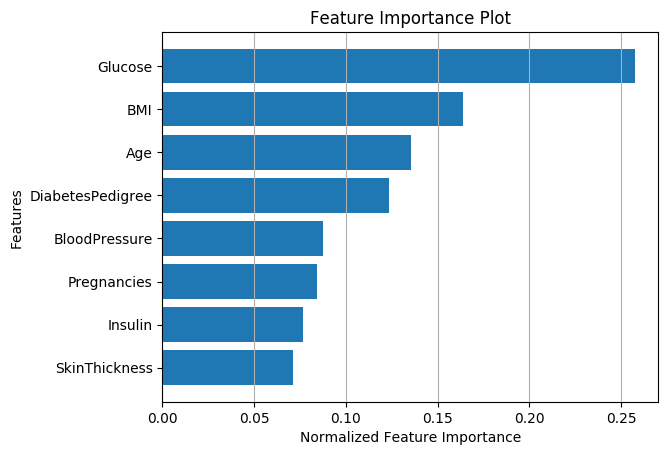
Feature Importance

This uses the feature_importances_ attribute of the ensemble methods in Scikit Learn which is calculated by the Mean Decrease in Impurity (MDI).

$ni_j=w_jC_j - w_{left(j)}C_{left(j)} - w_{right(j)}C_{right(j)}$ where

$ni_j=$ The importance of node $j$,

$w_j$ = The weight of samples reaching node $j$,

$C_j$ = The impurity of node $j$,

$left(j)$ = The child node from left split on node $j$,

$right(j)$ = The child node from right split on node $j$,

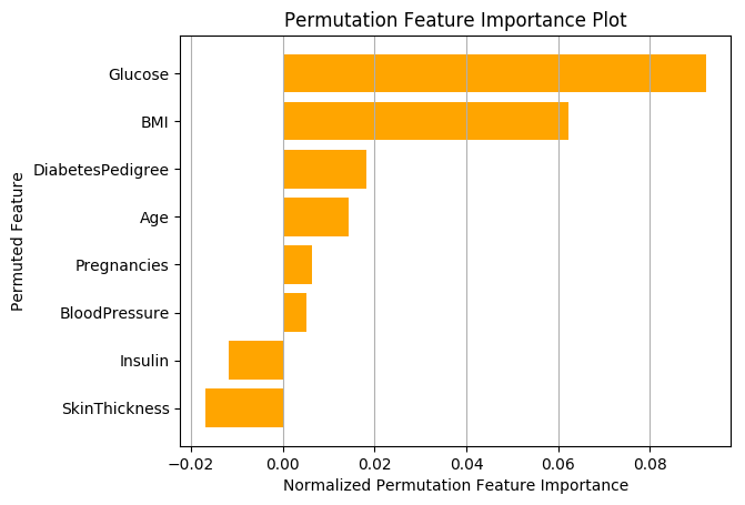
Feature Permutations

Here, for each feature in $(X_1, X_2, ..., X_n)$ the feature $(X_i)$ is permuted (values are shuffled randomly), the model is retrained and the mean drop in accuracy (MDA) is measured to ascertain the importance of the feature. This was also performed on the Diabetes Dataset.

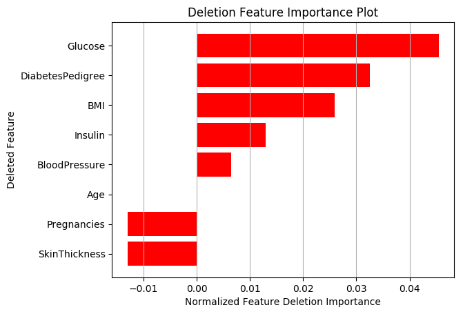
Feature Deletions

Here, for each feature in $(X_1, X_2, ..., X_n)$ the feature $(X_i)$ is completely deleted, the model is retrained and the mean drop in accuracy (MDA) is measured to ascertain the importance of the feature. This was done on the Diabetes Dataset.

Individual Conditional Expectations

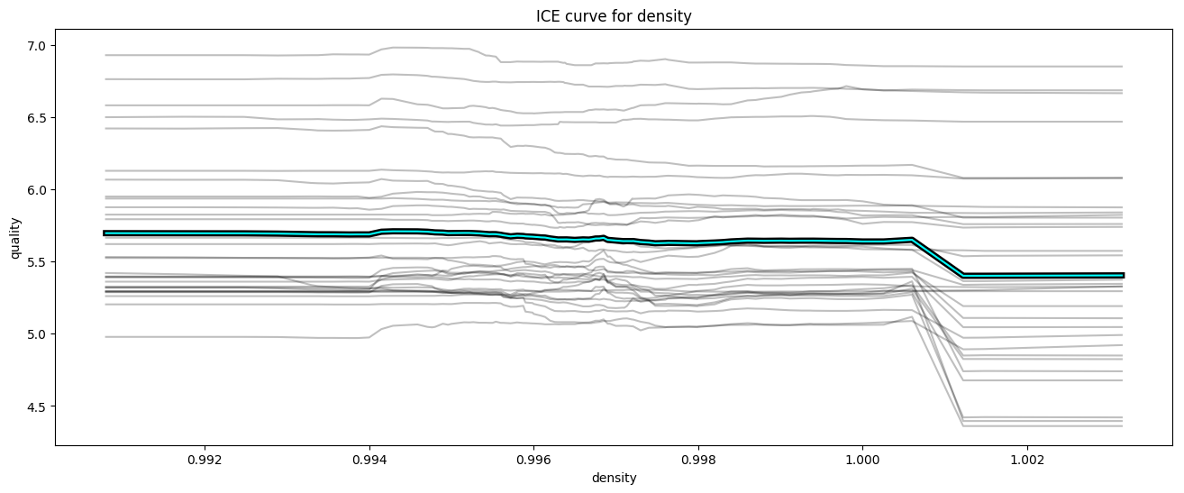
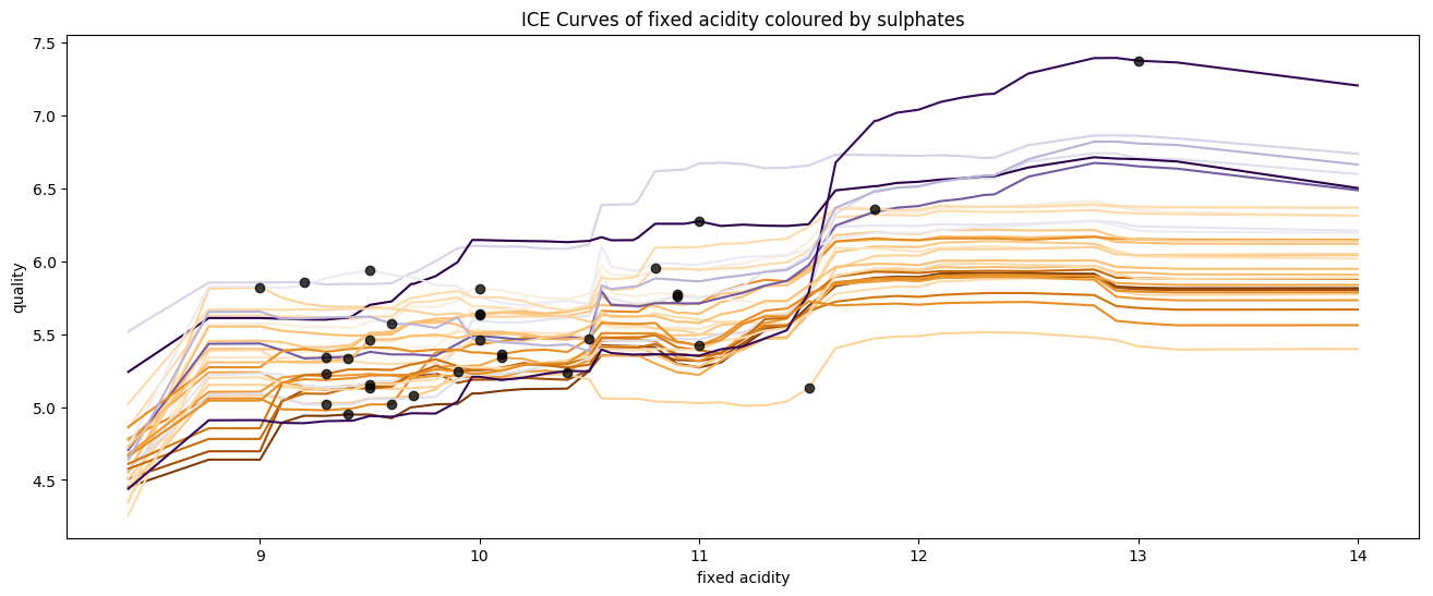
Individual Conditional Expectation (ICE) are a local per-instance method really useful in revealing feature interactions. They display one line per instance that shows how the instance’s prediction changes when a feature changes.

Formally, in ICE plots, for each instance in ${(x_S^{(i)}, x_C^{(i)})}_{i=1}^N$ the curve $\hat{f}_S^{(i)}$ is plotted against $(x_S^{(i)})$ while $(x_C^{(i)})$ remains fixed.

The $x_S$ are the feature vectors for which the ICE must be plotted and $x_C$ are the other features used in the underlying machine learning model $\hat{f}$

In these examples, the underlying model $\hat{f}$ used is a RandomForestRegressor

Examples from the Wine Quality Dataset are shown below.

Partial Dependence Plots

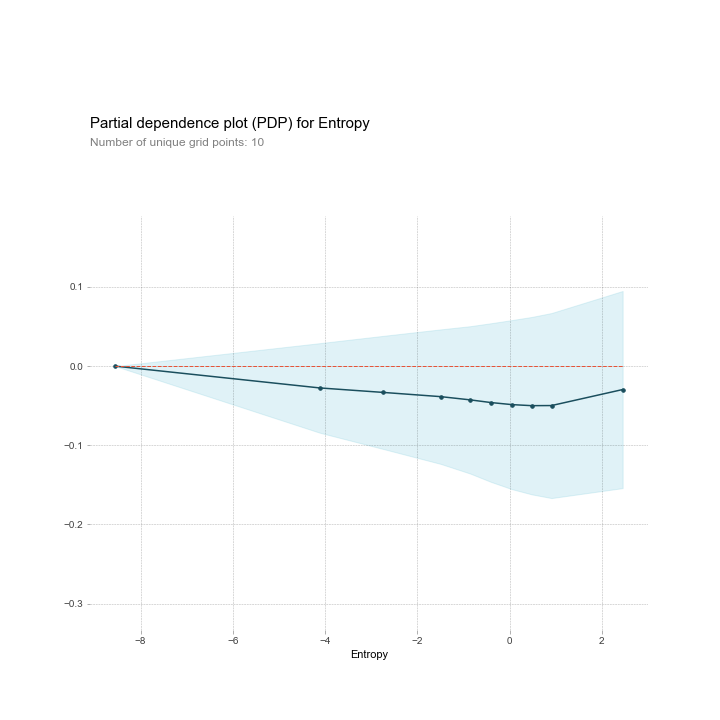
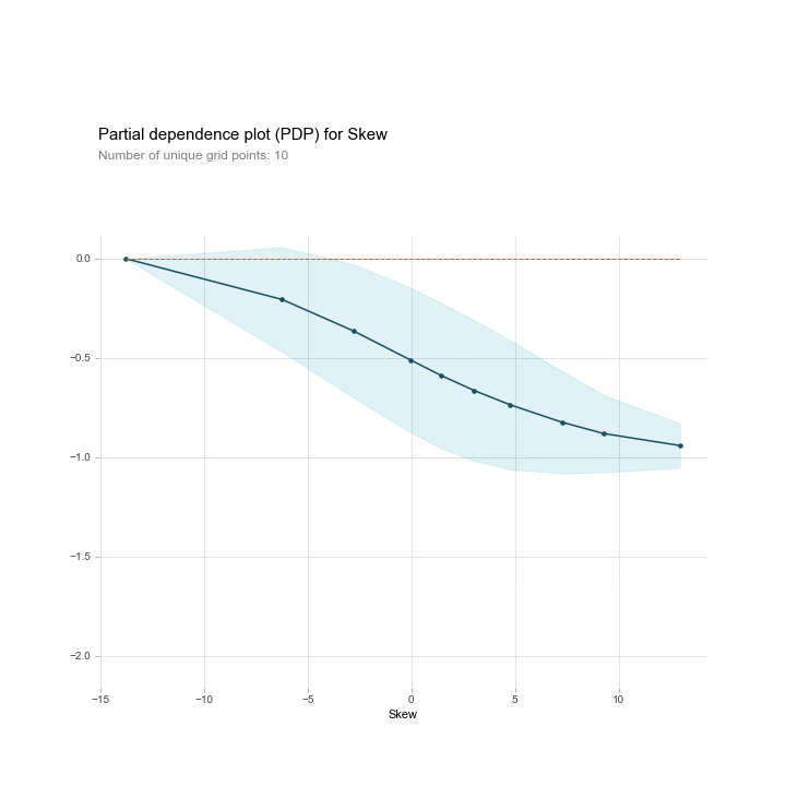
Partial dependence plots (short PDP or PD plot) shows the marginal effect one or two features have on the predicted outcome of a machine learning model. A partial dependence plot can show whether the relationship between the target and a feature is linear, monotonic or more complex.

For regression, the partial dependence function is:

Again, $x_S$ are the feature vectors for which the ICE must be plotted and $x_C$ are the other features used in the underlying machine learning model $\hat{f}$ and the set $S$ which is usually small and consists only of one or two features.

The partial function $\hat{f}_{x_S}$ is calculated as follows:

$$ \hat{f}_{x_S}(x_S) = \frac{1}{n} \sum_{i=1}^n \hat{f}(x_S, x_C^{(i)}) $$

The partial function tells us for given value(s) of features $S$ what the average marginal effect on the prediction is.

The underlying model $\hat{f}$ used here is a shallow (1 hidden layer) Neural Network, an MLPClassifier with around 25 neurons in the hidden layer and the dataset used is the BankNotes Authentication Dataset.

Shapley Values

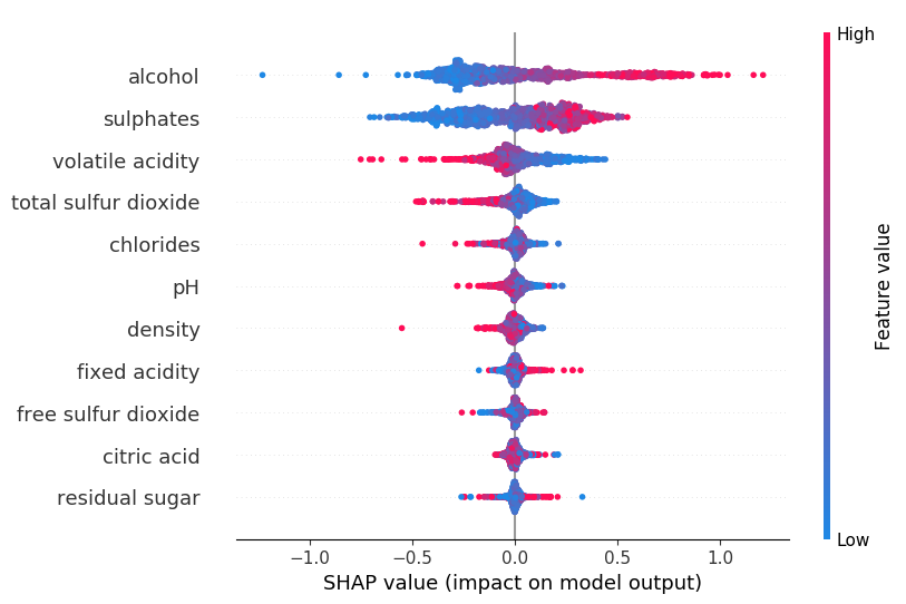
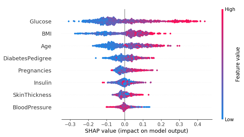
This idea comes from game theory and gives a theoretical estimate of feature prediction as compared to the above methods which were empirical and also gives importance to the sequence of features introduced.

The contribution of feature $i$ given the value function or underlying model $v$ is given as follows:

$\phi_i(v)=\sum_{S \subseteq (N \backslash {i})}\frac{|S|!(|N| - |S| - 1)!}{|N|!} (v(S\cup{{i}}) - v(S))$

where $S$ is a subset of the feature set $N$ and $v(S)$ gives the total model contribution of the subset $S$.

The underlying model $v$ used for this experiment is a RandomForestRegressor on the Diabetes and the Wine Quality datasets.

Diabetes Dataset

Wine Quality Dataset

Local Interpretable Model-Agnostic Explanations

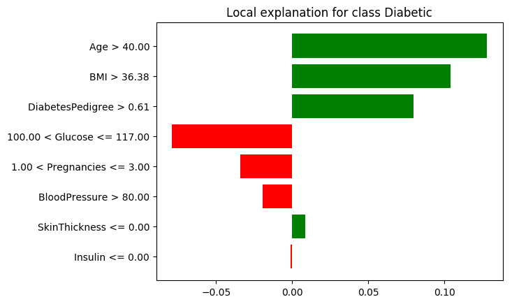
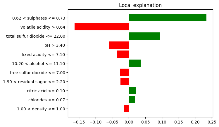
Local Interpretable Model-Agnostic Explanation (LIME) is a black-box model agnostic technique, which means it is independent of the underlying model used. It is however, local in nature, and generates an approximation and explanation for each example/instance of data. The explainer tries to perturb model inputs which are more interpretable to humans and then tries to generate a linear approximation locally in the neighbourhood of the prediction.

In general, the overall objective function is given by

$\xi(x)=argmin_{g \in G}\mathcal{L}(f, g, \pi_x) + \Omega(g)$

where $g(x)$ is the explainer function/model,

$\pi_x$ defines the locality/neighbourhood,

$\mathcal{L}$ defines the deviation or loss (or unfaithfulness) from the predictions of the actual model $f$,

$G$ is the class/family of explainable functions.

These are better illustrated by examples: (Examples on the Diabetes and the Wine Quality datasets)

Probability of being Diabetic: 0.56

Prediction: Diabetic

Predicted Wine Quality: 5.8 / 10

bharatr21/eXplAIners