Exploring Text Summarization Techniques
Text Summarization is the task of generating a short and concise summary that captures the main ideas of the source text. There are two main approaches to text summarization:
Abstractive methods build an internal semantic representation of the original content, and then use this representation to create a summary that is closer to what a human might express.
The generated summaries potentially contain new phrases and sentences that may not appear in the source text.
The current state of the art can be tracked here
Extractive methods use the original text to create a summary that is as close as possible to the original content. Here, content is extracted from the original data, but the extracted content is not modified in any way.
Most of the techniques explored in this project are related to extractive summarization.
The current state of the art can be tracked here
The main set of metrics used to evaluate the performance of text summarization techniques are ROUGE (Recall-Oriented Understudy for Gisting Evaluation) of which we use the following:
where
We use the sumeval package which implements this method.
An alternative implementation of the metric which uses precision, recall and F-measures provided by the rouge package in Python is as follows:
Precision
Recall
rouge and sumeval packages use the same implementation as follows:
Precision
Recall
and F-score
where
NOTE: A lot of the baselines explained here are implemented with the sumy package in Python.
This method is a variation of TF-IDF where the centroid is the average of the TF-IDF scores of all the words in the text.
The simple version of the TF-IDF formula is as follows:
For term
where
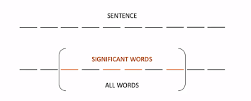
This method can be extended to use abstracts/excerpts instead of complete sentences and works as follows:
- First identify the sentence which consists of the cluster containing the maximum number of significant words. (This can be determined by another frequency based algorithm such as TF-IDF or thresholding)
- Significance of Sentence =
$\frac{[Count( significant\ words\ in\ sentence)]^2}{Count(words\ in\ sentence)}$
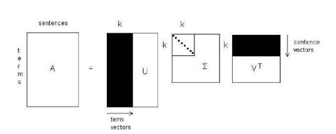
Latent Semantic Analysis (LSA) applies the concept of Singular Value Decomposition (SVD) to text summarization.
A term by sentence matrix
where
Σ is an
For each sentence vector in matrix
Formally:
where
TextRank is a graph-based model for many NLP applications, where the importance of a single sentence depends on the importance of the entire document, and with respect to other sentences in a mutually recursive fashion, similar to HITS or PageRank.
The score of a “text unit” or vertex
For the task of sentence (summary) extraction, the goal is to rank entire sentences, and therefore a vertex is added to the graph for each sentence in the text. Two sentences are connected if there is a “similarity” relation between them, where “similarity” is measured as a function of their content overlap (common tokens). For two sentences
where
TextRank takes into account both the local context of a text unit (vertex) and the information recursively drawn from the entire text document (graph).
This could be enhanced by considering the text units as words and then giving an improved similarity score to the sentences by considering PageRank scores of tokens between
Another graph-based model for many NLP applications, this method performs random walks or random traversals through the graph, where the lexical unit or vertex
Here, the similarity score between two sentences
where
and
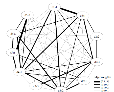
This is an example of a weighted-cosine similarity graph generated for a cluster where
We proposed a new algorithm BigramRank as a new graph based model which considers the basic lexical unit as bigrams (two consecutive tokens/words). This considers the frequency of bigrams (two consecutive words) and assigns the sentence relevance score for a sentence
Sentence Relevance Score of
This is the graph generated for the sentences “Windows 7 is a bit faster. Windows 7 is a little faster.” The bigram (Windows, 7) occurs 2 times, (little, faster) occurs 1 time.
The bigrams at the beginning and end of the sentence are considered slightly more important than bigrams occurring at the middle of a sentence, under the assumption that human readers may just skim through the beginning and end of a large sentence to look for the meaning of what the sentence conveys. To do this, the existing bigram frequency weights are multiplied elementwise by a kernel, which is
Eg: - Kernel of length 5 is
This assumes the opposite, that is, when humans read a sentence, they may tend to skip to the middle part of a sentence to get information and the beginning is full of transition words/conjunctions. In this case, the rest of the algorithm remains same and the kernel gets flipped to
Eg: - Kernel of length 5 is
This is based on the fact that the
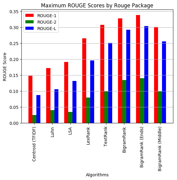
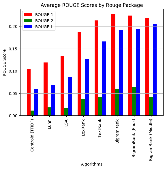
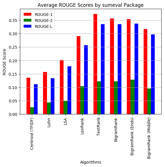
The metrics were measured in two ways, each with both the sumeval and rouge packages for each document and then averaged over all documents.
- The average ROUGE scores with all the available gold standard summaries were taken (on-average performance) for each document.
- The maximum ROUGE score of the available gold summaries (of a document) was taken to be the ROUGE score (for that document) (max performance).
| Algorithm | ROUGE-1 | ROUGE-2 | ROUGE-L |
|---|---|---|---|
| Centroid (TFIDF) | 0.149 | 0.025 | 0.087 |
| Luhn | 0.172 | 0.040 | 0.106 |
| LSA | 0.192 | 0.034 | 0.131 |
| LexRank | 0.265 | 0.080 | 0.196 |
| TextRank | 0.308 | 0.099 | 0.251 |
| BigramRank | 0.328 | 0.134 | 0.292 |
| BigramRank (Ends) | 0.338 | 0.140 | 0.303 |
| BigramRank (Middle) | 0.301 | 0.100 | 0.255 |
| Algorithm | ROUGE-1 | ROUGE-2 | ROUGE-L |
|---|---|---|---|
| Centroid (TFIDF) | 0.104 | 0.011 | 0.058 |
| Luhn | 0.119 | 0.018 | 0.068 |
| LSA | 0.134 | 0.016 | 0.086 |
| LexRank | 0.186 | 0.037 | 0.127 |
| TextRank | 0.213 | 0.042 | 0.166 |
| BigramRank | 0.227 | 0.060 | 0.191 |
| BigramRank (Ends) | 0.224 | 0.064 | 0.193 |
| BigramRank (Middle) | 0.219 | 0.042 | 0.205 |
| Algorithm | ROUGE-1 | ROUGE-2 | ROUGE-L |
|---|---|---|---|
| Centroid (TFIDF) | 0.135 | 0.026 | 0.112 |
| Luhn | 0.156 | 0.043 | 0.133 |
| LSA | 0.202 | 0.049 | 0.179 |
| LexRank | 0.290 | 0.104 | 0.257 |
| TextRank | 0.373 | 0.122 | 0.335 |
| BigramRank | 0.356 | 0.122 | 0.335 |
| BigramRank (Ends) | 0.354 | 0.128 | 0.337 |
| BigramRank (Middle) | 0.317 | 0.096 | 0.297 |
| Algorithm | ROUGE-1 | ROUGE-2 | ROUGE-L |
|---|---|---|---|
| Centroid (TFIDF) | 0.089 | 0.011 | 0.073 |
| Luhn | 0.105 | 0.019 | 0.092 |
| LSA | 0.138 | 0.020 | 0.122 |
| LexRank | 0.189 | 0.038 | 0.166 |
| TextRank | 0.248 | 0.053 | 0.229 |
| BigramRank | 0.241 | 0.051 | 0.228 |
| BigramRank (Ends) | 0.235 | 0.052 | 0.222 |
| BigramRank (Middle) | 0.219 | 0.042 | 0.205 |
