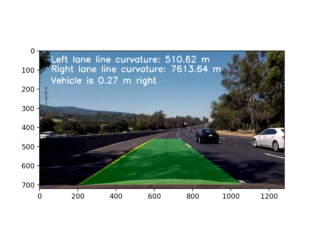
In this project, the goal is to write a software pipeline to identify the lane boundaries in a video from a front-facing camera on a car.
- Compute the camera calibration matrix and distortion coefficients given a set of chessboard images.
- Apply a distortion correction to raw images.
- Use color transforms, gradients, etc., to create a thresholded binary image.
- Apply a perspective transform to rectify binary image ("birds-eye view").
- Detect lane pixels and fit to find the lane boundary.
- Determine the curvature of the lane and vehicle position with respect to center.
- Warp the detected lane boundaries back onto the original image.
- Output visual display of the lane boundaries and numerical estimation of lane curvature and vehicle position.
- OpenCV — a computer vision library,
- Matplotlib — a python 2D plotting library,
- Numpy — a package for scientific computing with Python,
- MoviePy — a Python module for video editing.
The camera calibration is important in removing the radial distortion and tangential distortion. In radial distortion the straight lines will appear curved and in tangential distortion which occurs because image taking lens is not aligned perfectly parallel to the imaging plane. So some areas in image may look nearer than expected.
OpenCV has a built in API cv2.calibrateCamera() for calibrating cameras.
The function takes as input parameters an array of chessboard images. The images are read by using cv2.imread() function,
converts the images to grayscale using cv2.cvtColor(), then it finds the chessboard corners using cv2.findChessboardCorners().
Finally, the cv2.calibrateCamera() function is used to calibrate camera.
The values obtained by using the cv2.calibrateCamera() function will be used later to undistort images.
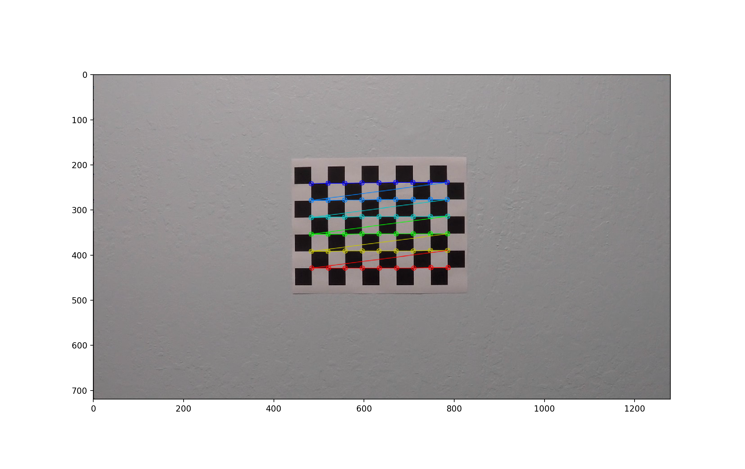
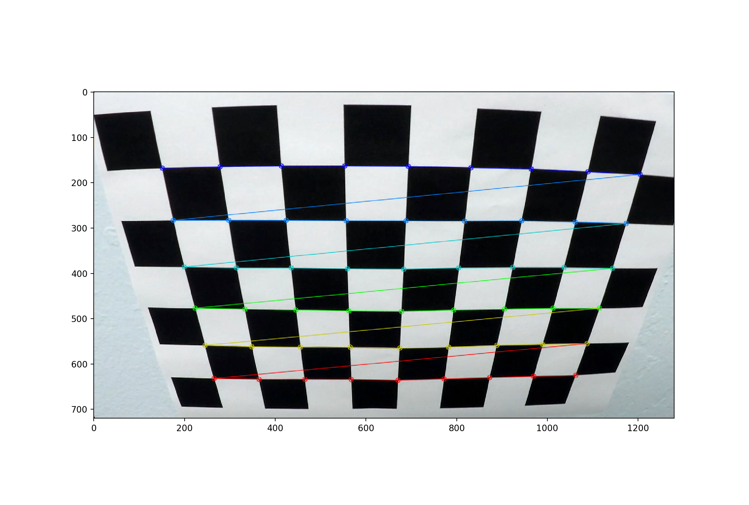
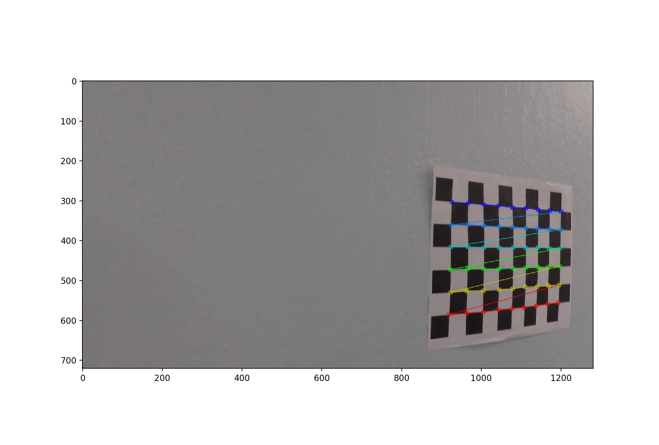
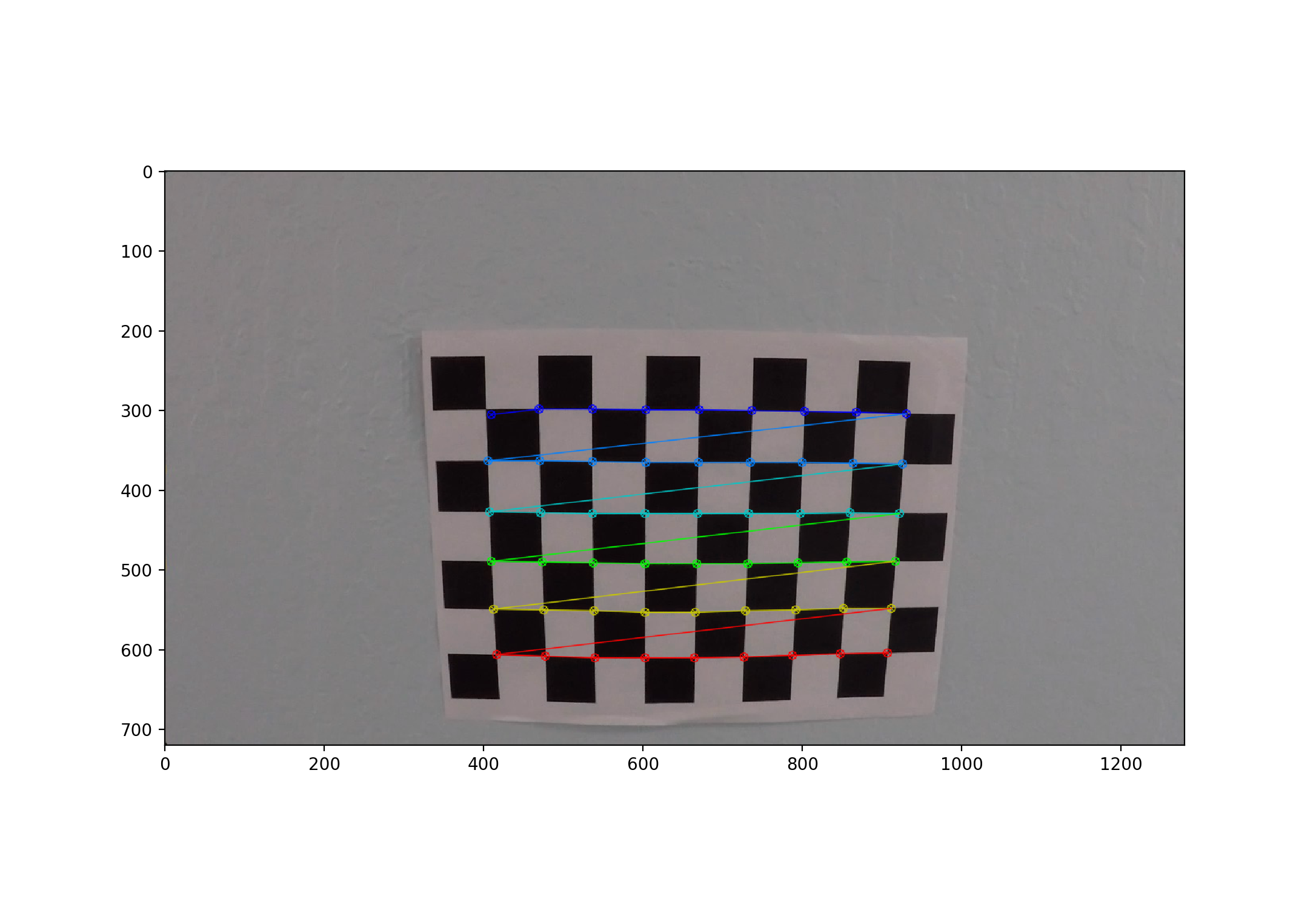
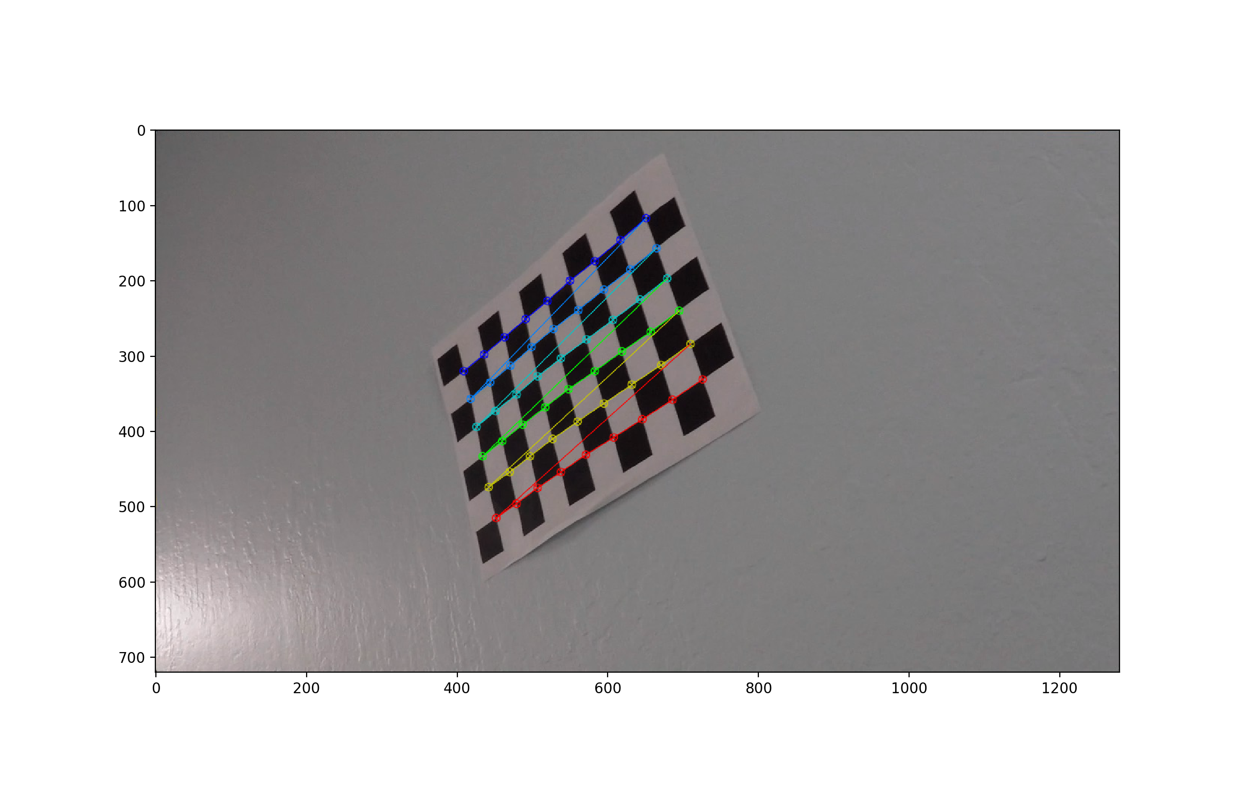
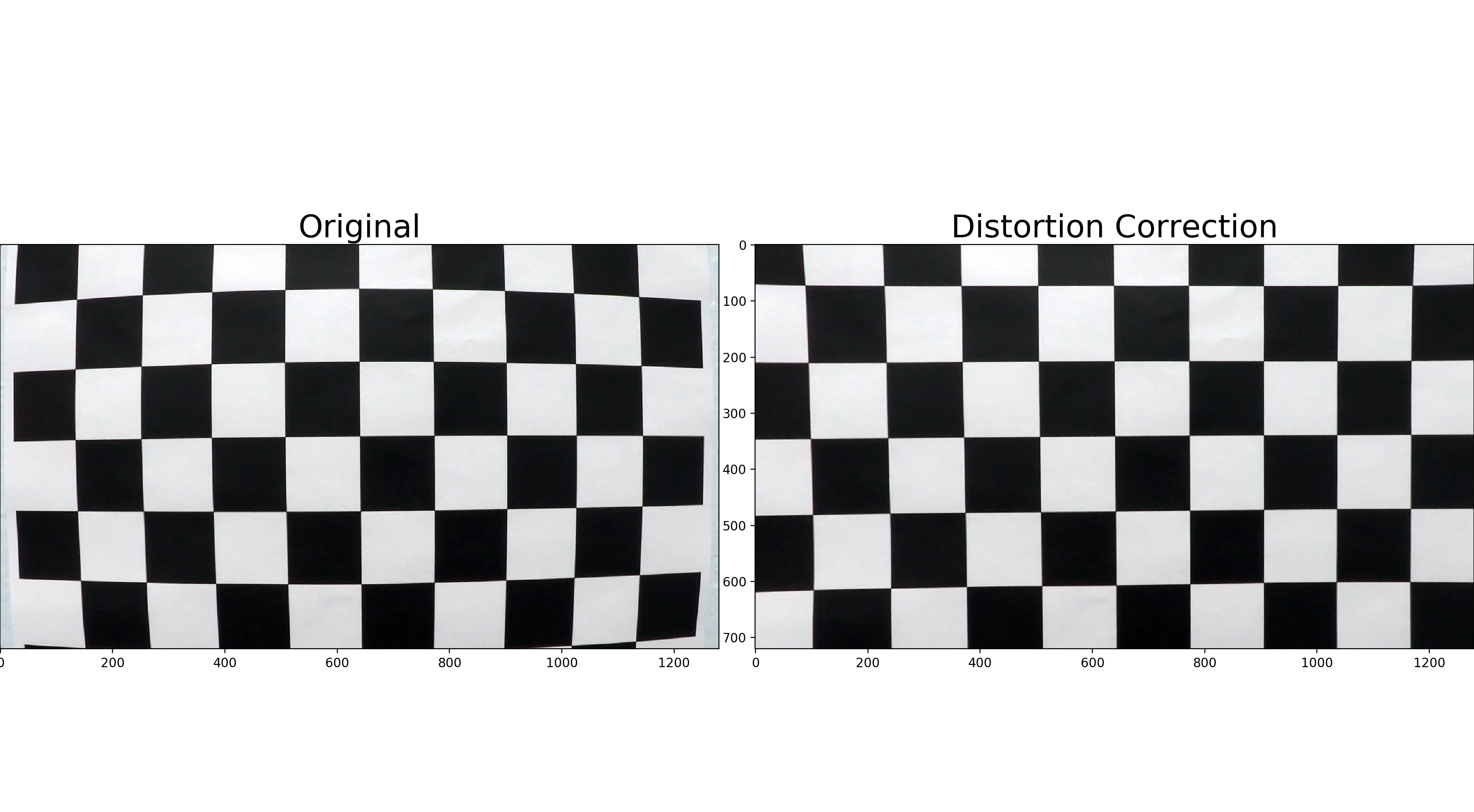
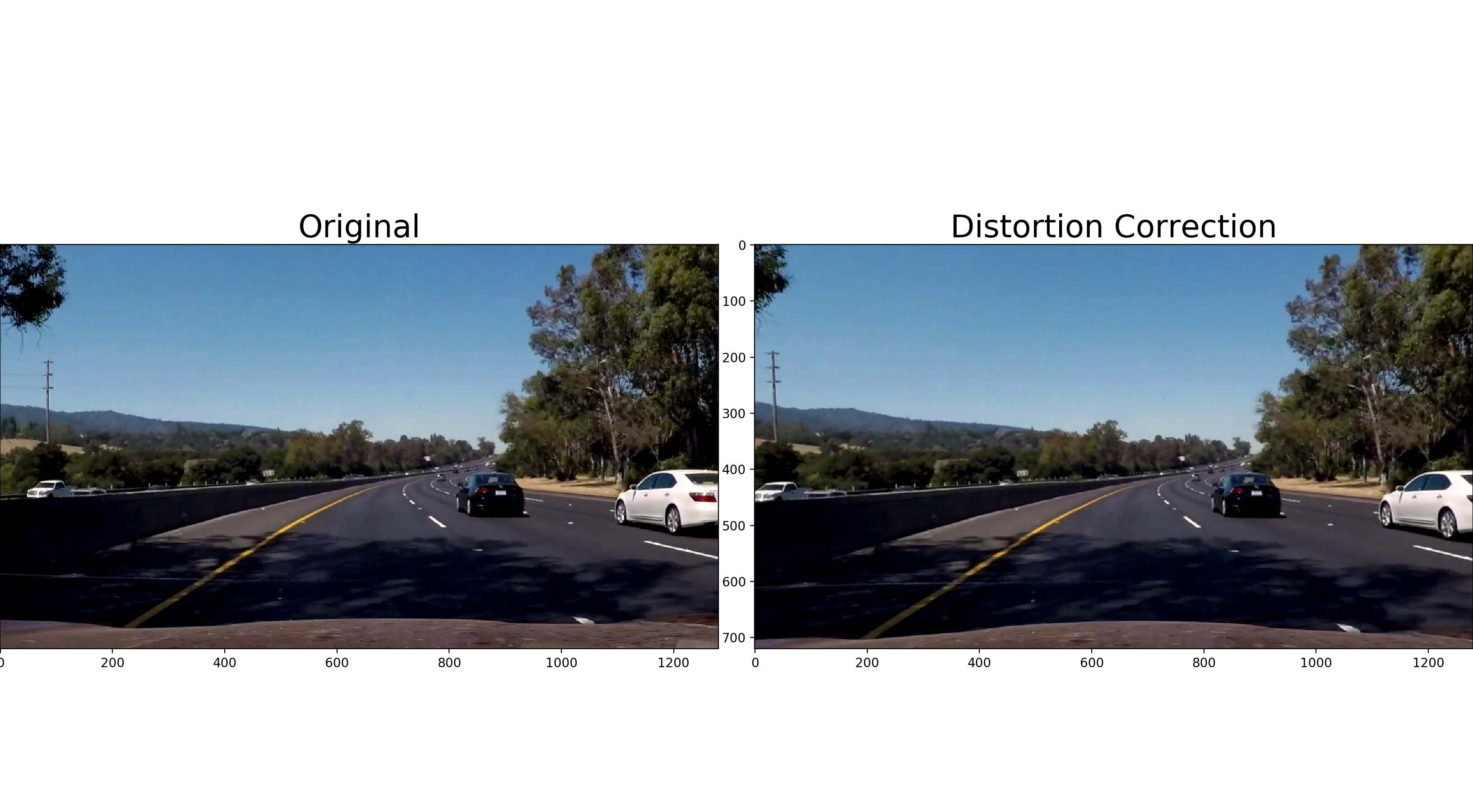
After obtaining mtx and dist parameters from the cv2.calibrateCamera function, now we can take an image and undistort
it using OpenCV function cv2.undistort()
Many various combination of color and gradient thresholds to generate a binary image where the lane lines are clearly visible are used.
Gradient on x and y direction, magnitude of the gradient, direction of the gradient, and color (HLS) transformation technique are used to obtain the final binary image.
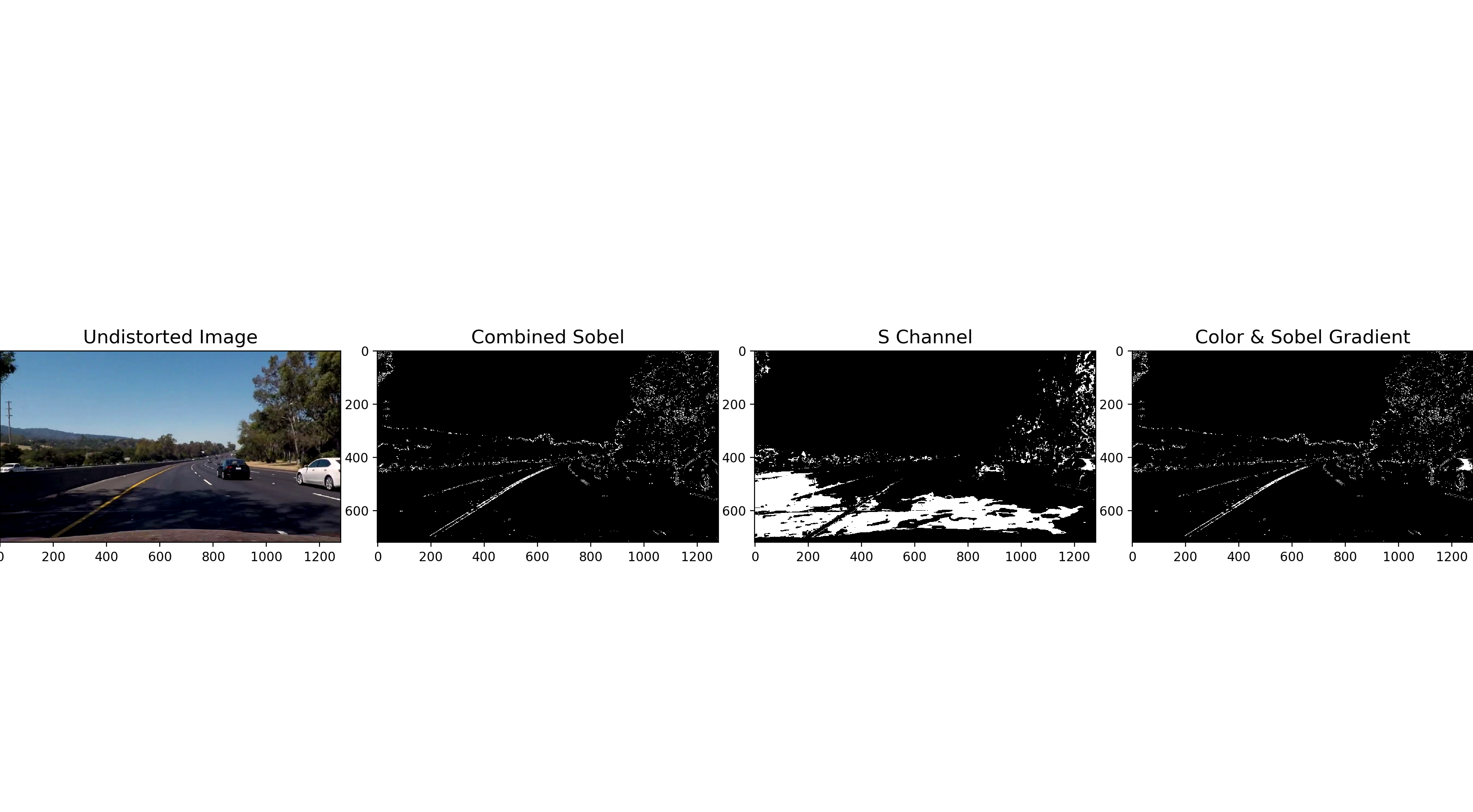
A perspective transform maps the points in a given image to different, desired, image points with a new perspective. The perspective transform you’ll be most interested in is a bird’s-eye view transform that let’s us view a lane from above; this will be useful for calculating the lane curvature.
OpenCV provide two functions cv2.getPerspectiveTransform() and cv2.warpPerspective() to perform this task.
I chose to hardcode the source and destination points in the following manner:
| Source | Destination |
|---|---|
| 280, 700 | 250, 720 |
| 595, 460 | 250, 0 |
| 725, 460 | 1065, 0 |
| 1125, 700 | 1065, 720 |
I verified that my perspective transform was working as expected by drawing the src and dst points onto a test image and its warped counterpart to verify that the lines appear parallel in the warped image.
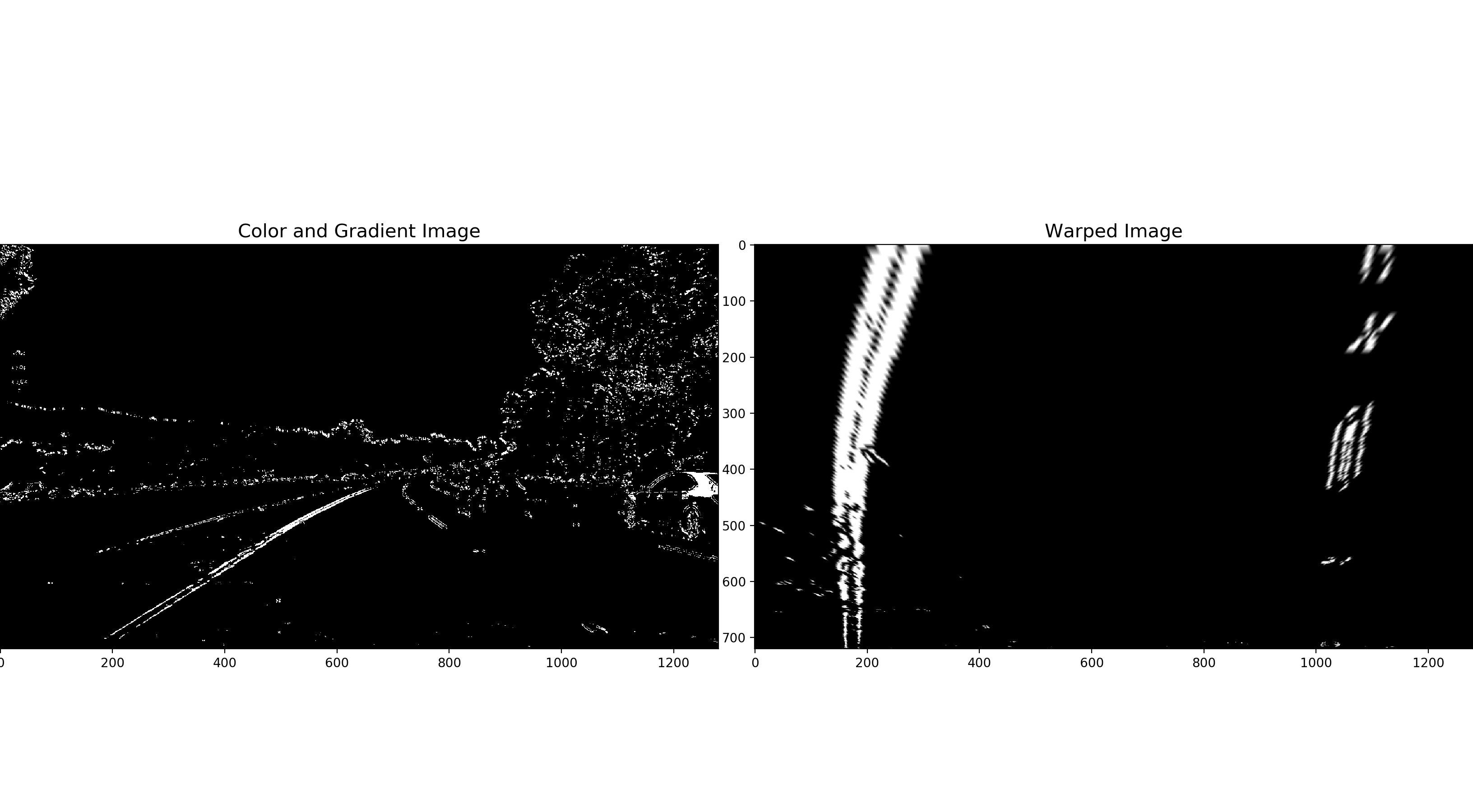
After applying calibration, thresholding, and a perspective transform to a road image, I now have a binary image where the lane lines stand out clearly. However, I still need to decide explicitly which pixels belong to the left line and which belong to the right line.
Plotting a histogram of where the binary activations occur across the image is one potential solution for this.
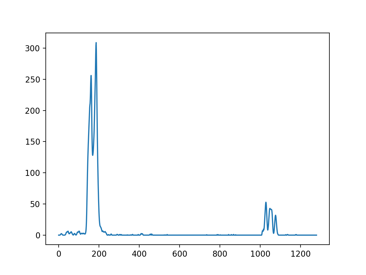
With the histogram I am adding up the pixel values along each column in the image. In thresholded binary image,
pixels are either 0 or 1, so the two most prominent peaks in the histogram will be good indicators of the x-position
of the base of the lane lines. I used that as a starting point for where to search for the lines. From that point,
I used a sliding window, placed around the line centers, to find and follow the lines up to the top of the frame.
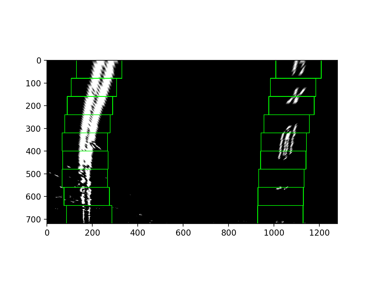
Now that I have found all our pixels belonging to each line through the sliding window method, it's time to fit a
polynomial to the line. Numpy’s function np.polyfit() will be used to calculate the polynomials.
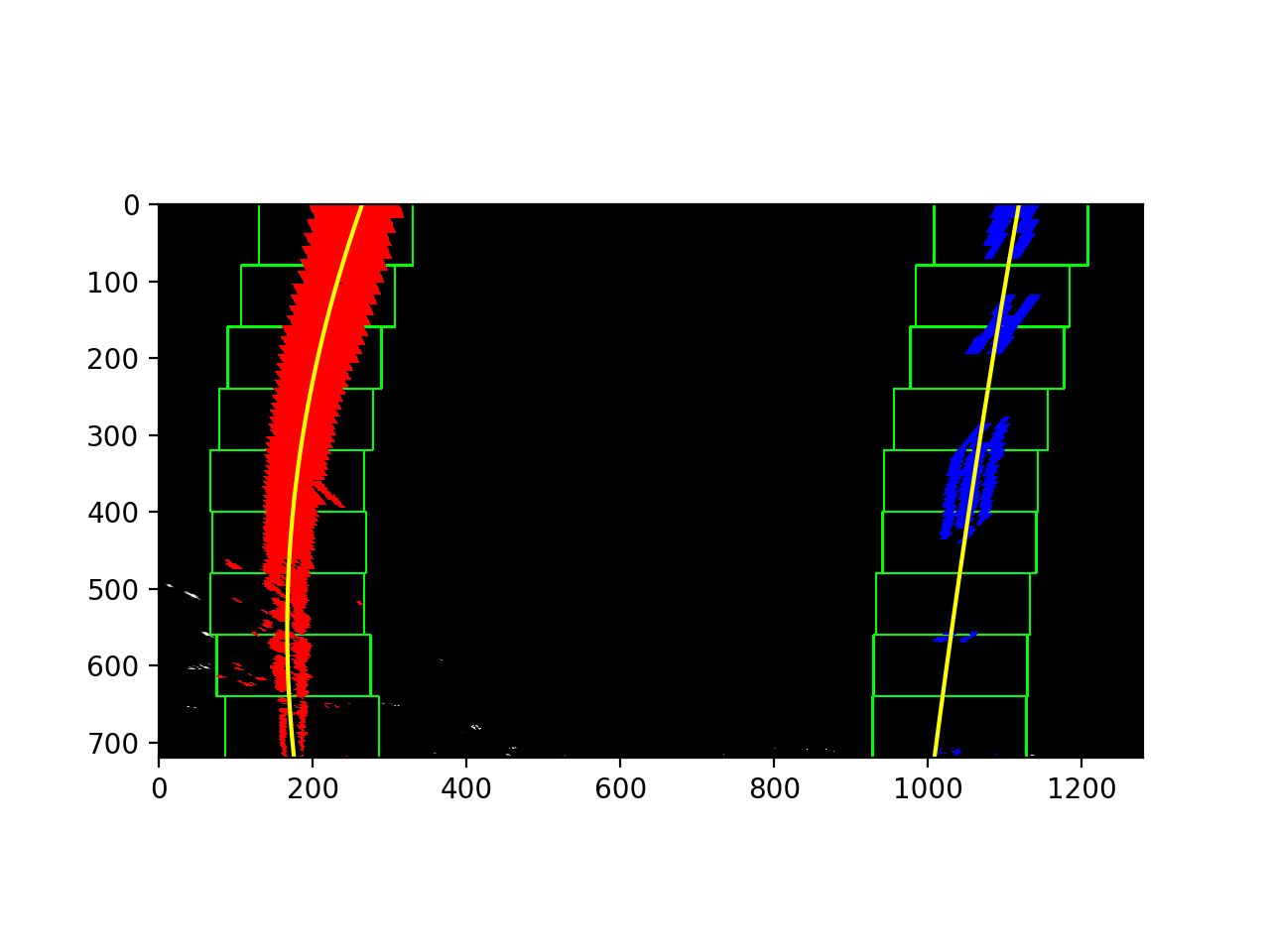
Once I have selected the lines, it is reasonable to assume that the lines will remain there in future video frames.
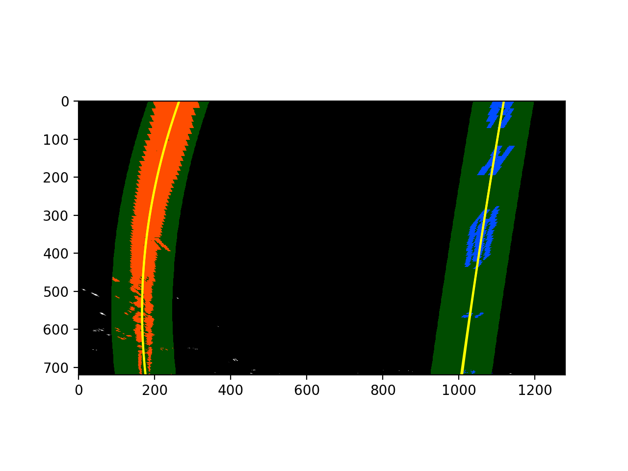
In the next frame of video I don't need to do a blind search again, but instead I can just search in a margin
around the previous lane line position. The green shaded area shows where we searched for the lines this time.
So, once I know where the lines are in one frame of video, I can do a highly targeted search for them in the next frame.
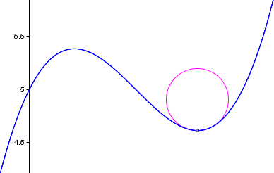
The radius of curvature of the curve at a particular point is defined as the radius of the approximating circle. This radius changes as we move along the curve.
We can draw a circle that closely fits nearby points on a local section of a curve, as follows.
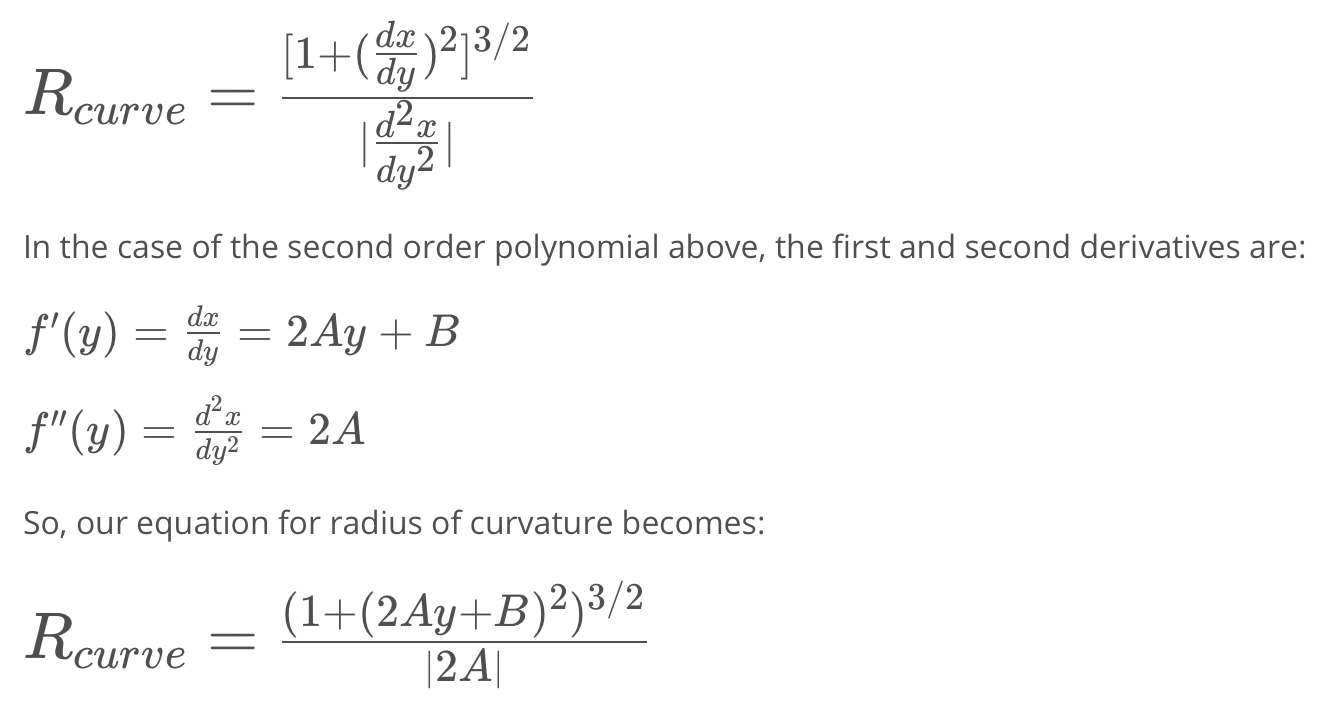
The radius of curvature at any point x of the function x=f(y) is given as follows:
The pipeline fails to perform well on challenge videos dues to changing in brightness and sharp curvature of the road.
Another issues I encounter was the lines under the shadow were not detected so I had to implement an additional color threshold (Lightness channel) to view the lanes clearly under the shadow.
