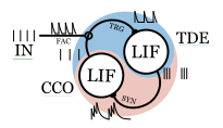
The repository containing the code used in the paper "Mastella, M., Tiemens, T. & Chicca, E. Texture Recognition Using a Biologically Plausible Spiking Phase-Locked Loop Model for Spike Train Frequency Decomposition 2024. arXiv: 2403.09723 [q-bio]" If this work helps you in your research consider citing it from here: https://arxiv.org/abs/2403.09723
The paper is divided in four different experiments.
The first experiment shows the behaviour of a single sPLL layer against different input frequencies.
The code generating the Figure 1 is contained in the Jupyter Notebook: Fig1_spll.ipynb.
In this code is also provided an incremental explanation on how the sPLL works.
Furthermore, we show how to generate the potential well described in the paper.
Running the code generates the two parts of the plot.
The second experiment shows instead how the architecture responds when recording from biological data from Macaque is presented.
The code generating the Figure 2 is contained in the Jupyter Notebook: Fig2_bio.ipynb
The data used for the input signals are obtained from the authors of the two following publications.
- Weber, A. I. et al. Spatial and temporal codes mediate the tactile perception of natural textures. PNAS 110, 17107–17112 (2013).
- Lieber, J. D. & Bensmaia, S. J. High-dimensional representation of texture in somatosensory cortex of primates. Proc Natl Acad Sci USA 116, 3268–3277 (2019).
For accessing said data please refer to the authors of said papers.
The third experiment compare the sPLL network against a linear classifier, a LSTM, a 1-layer recurrent LIF neural network trained with backpropagation and a 2-layer recurrent neural network trained in the same way.
The different networks are trained using the same parameters but different codes.
All codes have a training code (*_multifreq.py), a multiseed version (*_multifreq_seeds.py), a testing (*_multifreq_finalmodel.py).
The resulting values of accuracy, spike number and others was then sourced by the code Fig3_comp.ipynb
The input dataset is generated using the SPLL_dataset.py script.
The frequency, noise and other parameters related with said dataset are the default one for the script used.
The sPLL network is simulated in the SPLL_dataset.py script. In this we create a dataset of responses of the sPLL for all the inputs of the dataset.
The responses are then sourced by SPLL_notrain_multifreq.py in which a linear classifier gets trained. The trained classifier is then saved.
This part is repeated for 20 seeds using the code SPLL_notrain_multifreq_seeds.py
The code SPLL_notrain_multifreq_finalmodel.py runs the trained model (sPLL with linear classifier) saving number of spikes in total, accuracy and other metrics for every seed.
For the other networks, the data were directly pulled in the *_multifreq.py. Null, LSTM and LIF were the terms used for the linear classifier, the LSTM and the DSNN respectively.
For the DSNN the layer size was defining if the network was a single layer LIF (50) or a two layer LIF (50-50) in the argument --layers_size.
For the DSNNs the network was optimized using NNI.
The code running the NNI can be found in the script HPO.py.
The resulting optimized elements are called LIF_multifreq_[50]_opt.txt and LIF_multifreq_[50-50]_opt.txt and are sourced by the LIF_multifreq.py during the training.
The dataset used to train this was created with other seeds.
The search space can be found in LIF_multifreq_search.txt
In the forth experiment, presented in the supplementary materials, the same input data of the third experiment is analyzed using an histrogram of the interspike interval and a Fourier transform.
The code to visualize the result is Fig_S1_isi_vs_fft.ipynb, while the code generating it is isi_vs_fft.py
The resulting data can be found on:
