cyclingResults

Analyze cycling results from road results and USA cycling.

Installation

remotes::install_github('bill-ash/cyclingResults')
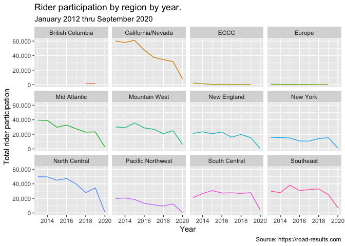
library(cyclingResults)

Example

Compare rider participation by region over time.

library(dplyr)
library(ggplot2)

road_results <- cyclingResults::get_races() 

road_results %>% 
  group_by(date, region, .drop = FALSE) %>% 
  mutate(date = lubridate::floor_date(date, 'year')) %>% 
  summarise(total = sum(racers)) %>% 
  filter(date > '2012-01-01') %>% 
  ggplot(aes(date, total, color = region)) + 
  geom_line() + 
  scale_y_continuous(labels = scales::comma_format()) +
  labs(title = 'Rider participation by region by year.', 
       subtitle = 'January 2012 thru September 2020', 
       caption = 'Source: https://road-results.com',
       x = 'Year', y = 'Total rider participation') + 
  facet_wrap(~region, ) + 
  theme(legend.position = 'none')

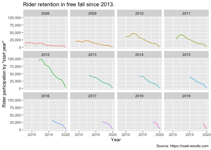
Explore rider retention over time. Load all race results from 2008 to 2020. raw_results() loads a .Rds file of all rider results scraped from road results.

library(cyclingResults)
library(tidyverse)

races_raw <- raw_results() %>% 
  mutate(license = readr::parse_number(license)) %>% 
  filter(!is.na(license), 
         nchar(license) > 4 & nchar(license) < 7,
         !license %in% c(91005, 999999))

races_raw %>%
  select(license, date) %>% 
  group_by(license, date = lubridate::floor_date(date, 'year')) %>% 
  count(date, license, sort = TRUE) %>% 
  ungroup() %>% 
  group_by(license) %>%
  # cohort is defined as the earliest date a license appears in the data
  mutate(cohort = min(date)) %>% 
  ungroup() %>% 
  group_by(cohort, date) %>% 
  # total participation by cohort, by year
  summarise(total = sum(n), 
            cohort = as.factor(lubridate::year(cohort))) %>% 
  filter(cohort != 2020) %>% 
  ggplot(aes(date, total, color = cohort)) + 
  geom_line() + 
  scale_y_continuous(labels = scales::comma_format()) + 
  labs(title = 'Rider retention in free fall since 2013.',
       x = 'Year', y = 'Rider participation by "start year"',
       caption = 'Source: https://road-results.com') + 
  facet_wrap(~cohort) + 
  theme(legend.position = 'none')

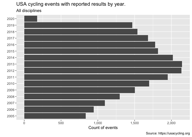
Analyze permit data from USA cycling with usa_permits().

library(cyclingResults)
library(dplyr)
library(ggplot2)

usa_cycling_permits <- cyclingResults::usa_permits() 

usa_cycling_permits %>% 
  group_by(year = as.factor(lubridate::year(race_date)), .drop = FALSE) %>% 
  summarise(total = n()) %>% 
  ggplot(aes(year, total)) + 
  geom_col() + 
  scale_y_continuous(labels = scales::comma_format()) +
  coord_flip() + 
  labs(title = 'USA cycling events with reported results by year.',
       subtitle = 'All disciplines',
       caption = 'Source: https://usacycling.org',
       x = '', y = 'Count of events')

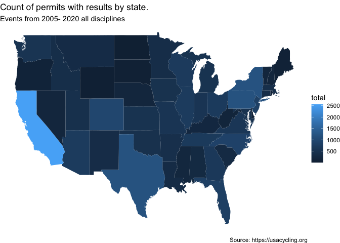
Make a map of permits with reported results by state. Each observation represents a permit that can have more than one event.

library(ggmap)
library(maps)
library(tidyverse)
library(cyclingResults)

states_map <- map_data('state')

cyclingResults::usa_permits() %>% 
  group_by(state) %>%
  summarise(total = n()) %>% 
  inner_join(setNames(bind_cols(tolower(state.name), state.abb),
                      c('region', 'state'))
             ) %>%  
  ggplot(aes(map_id = region)) + 
  geom_map(aes(fill = total), map = states_map) + 
  expand_limits(x = states_map$long, y = states_map$lat) + 
  labs(title = 'Count of permits with results by state.', 
       subtitle = 'Events from 2005- 2020 all disciplines',
       caption = 'Source: https://usacycling.org') + 
  theme_void()

This package is still in development.