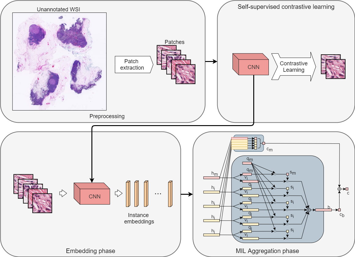
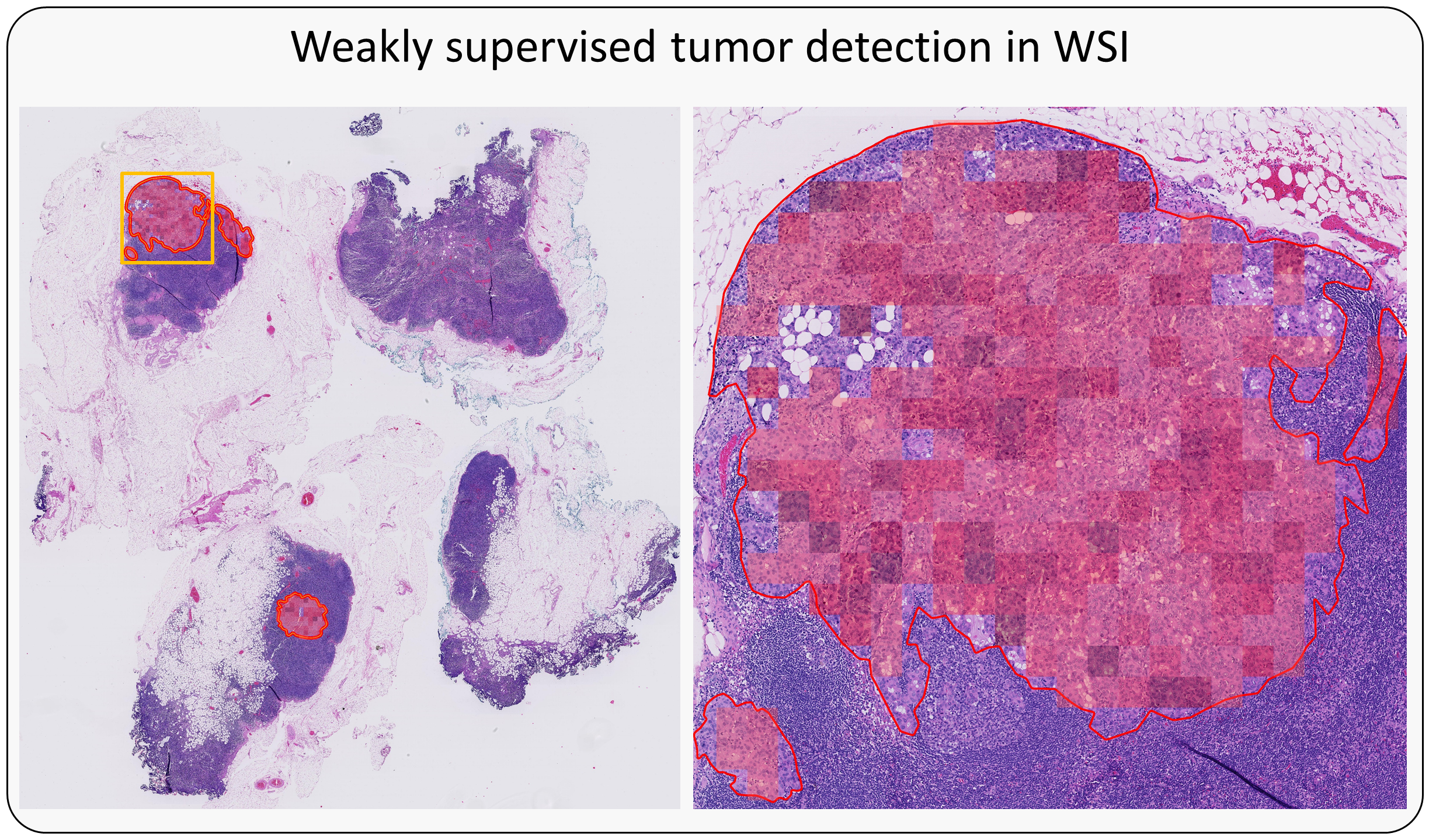
DSMIL: Dual-stream multiple instance learning networks for tumor detection in Whole Slide Image

Pytorch implementation for the multiple instance learning model described in the paper Dual-stream Multiple Instance Learning Network for Whole Slide Image Classification with Self-supervised Contrastive Learning (CVPR 2021, accepted for oral presentation).

Updates 2024

10x training speedup.
Cross-validation and train/valid/test (cross-validation + a standalone test set) in the training script.
A stable model initialization method.
Better metrics for multi-label tasks.
Several bugs fixed in scripts for generating color maps.

Installation

Install anaconda/miniconda
Required packages

  $ conda env create --name dsmil --file env.yml
  $ conda activate dsmil

Install PyTorch
Install OpenSlide and openslide-python.
Tutorial 1 and Tutorial 2 (Windows).

Download feature vectors for MIL network

MIL benchmark datasets can be downloaded via:

  $ python download.py --dataset=mil

Precomputed features for TCGA Lung Cancer dataset can be downloaded via:

  $ python download.py --dataset=tcga

Precomputed features for Camelyon16 dataset

  $ python download.py --dataset=c16

This dataset requires 30GB of free disk space.

Training on default datasets.

MIL benchmark datasets

Train DSMIL on standard MIL benchmark dataset:

  $ python train_mil.py

Switch between MIL benchmark dataset, use option:

[--datasets]      # musk1, musk2, elephant, fox, tiger

Other options are available for learning rate (--lr=0.0002), cross validation fold (--cv_fold=10), weight-decay (--weight_decay=5e-3), and number of epochs (--num_epoch=40).

WSI datasets

Train DSMIL on TCGA Lung Cancer dataset (precomputed features):

 $ python train_tcga.py --dataset=TCGA-lung-default

Train DSMIL on Camelyon16 dataset (precomputed features):

 $ python train_tcga.py --dataset=Camelyon16 --num_classes=1

Understanding different evaluation schemes and metrics

Different training and evaluation schemes can be choosen by setting the arugment (--eval_scheme).

--eval_scheme=5-fold-cv

A 5-fold cross-validation. For each fold, AUC and accuracy score will be computed on the validation set. Averaged values across the 5 folds will be computed after all folds complete.

--eval_scheme=5-fold-cv-standalone-test

A standalone test set consisting of 20% samples is reserved, remaining 80% samples are used to construct a 5-fold cross-validation.
For each fold, the best model and corresponding threshold are saved.
After the 5-fold cross-validation, 5 best models along with the corresponding optimal thresholds are obtained which are used to perform inference on the reserved test set. A final prediction for a test sample is the majority vote of the 5 models.
For a binary classification, accuracy and balanced accuracy score are computed. For a multi-label classification, hamming loss (smaller the better) and subset accuracy are computed.

Expected performance

You may see slightly different performance due to random splits but the difference should be about within 2%
Camelyon16 with a 5-fold cross-validation.

Metric	Accuracy	AUC
Values	94.9%	0.961

Camelyon16 with a 5-fold cross-validation and a standalone test set.

Metric	Accuracy	AUC
Values	92.4%	0.915

TCGA Lung with a 5-fold cross-validation.

Metric	Accuracy	AUC
Values	93.78%	0.981

TCGA Lung with a 5-fold cross-validation and a standalone test set.

Metric	Subset accuracy	Hamming loss
Values	90.9%	0.086

Useful arguments:

[--num_classes]       # Number of non-negative classes, for a binary classification (postive/negative), this is set to 1
[--feats_size]        # Size of feature vector (depends on the CNN backbone)
[--lr]                # Initial learning rate [0.0001]
[--num_epochs]        # Number of training epochs [50]
[--stop_epochs]       # Skip remaining epochs if training has not improved after N epochs [10]
[--weight_decay]      # Weight decay [1e-3]
[--dataset]           # Dataset folder name
[--split]             # Training/validation split [0.2]
[--dropout_patch]     # Randomly dropout a portion of patches and replace with duplicates during training [0]
[--dropout_node]      # Randomly dropout a portion of nodes in the value vector generation network during training [0]

Testing and generating detection maps from WSI

TCGA dataset

Download some testing slides:

  $ python download.py --dataset=tcga-test

You might need to unzip the file manually. 7-zip might be required for unzipping in Linux. To crop the WSIs into patches, run:

  $ python test_crop_single.py --dataset=tcga

A folder containing all patches for each WSI will be created at ./test/patches.
After the WSIs are cropped, run the testing script:

  $ python testing_tcga.py

The thumbnails of the WSIs will be saved in ./test/thumbnails.
The detection color maps will be saved in ./test/output.
The testing pipeline will process every WSI placed inside the ./test/input folder. The slide will be detected as a LUAD, LUSC, or benign sample.

Camelyon16 dataset

Generating detection maps for Camelyon16 is similar. Direct download link for the sample slides.

  $ python download.py --dataset=c16-test
  $ python test_crop_single.py --dataset=c16
  $ python testing_c16.py

Processing raw WSI data

If you are processing WSI from raw images, you will need to download the WSIs first.

Download WSIs.

From GDC data portal. You can use GDC data portal with a manifest file and configuration file. The raw WSIs take about 1TB of disc space and may take several days to download. Please check details regarding the use of TCGA data portal. Otherwise, individual WSIs can be download manually in GDC data portal repository
From Google Drive. The svs files are also uploaded. The dataset contains in total 1053 slides, including 512 LUSC and 541 LUAD. 10 low-quality LUAD slides are discarded.

Sort svs files in the folder. Separate LUAD and LUSC slides according to the IDs and place the files into folder WSI/TCGA-lung/LUAD or WSI/TCGA-lung/LUSC.

Prepare the patches.

We will be using OpenSlide, a C library with a Python API that provides a simple interface to read WSI data. We refer the users to OpenSlide Python API document for the details of using this tool.
The patches could be saved in './WSI/TCGA-lung/pyramid' in a pyramidal structure for two magnification levels. The first magnification level is level 0, which corresponds to a base magnification specified by -b. For example, to extract patches at 20x and 5x magnifications, run:

  $ python deepzoom_tiler.py -m 0 2 -b 20

Or, the patches could be cropped at a single level magnification and saved in './WSI/TCGA-lung/single'. For example, extract patches at 10x magnification:

  $ python deepzoom_tiler.py -m 0 -b 10

Camelyon16 consists of mixed magnifications so to reproduce:

 $ python deepzoom_tiler.py -m 1 -b 20 -d Camelyon16 -v tif

Train the embedder.

We provided a modified script from this repository Pytorch implementation of SimCLR For training the embedder.
Navigate to './simclr' and edit the attributes in the configuration file 'config.yaml'. You will need to determine a batch size that fits your gpu(s). We recommend using a batch size of at least 512 to get good simclr features. The trained model weights and loss log are saved in folder './simclr/runs'.
If patches are cropped in single magnification.

  cd simclr
  $ python run.py

If patches are cropped in multiple magnifications, the embedder for each magnification needs to be trained separately to achieve better results.

  $ python run.py --multiscale=1 --level=low
  $ python run.py --multiscale=1 --level=high

Otherwise, you could use the trained embedder for Camelyon16 and TCGA

Compute the features.

Compute the features for single magnification:

  $ cd ..
  $ python compute_feats.py --dataset=TCGA-lung

The last trained embedder will be used by default. To use a specific embedder, set the option --weights=[RUN_NAME], where [RUN_NAME] is a folder name inside simclr/runs/. Or, compute the features for multiple magnifications:

  $ python compute_feats.py --dataset=TCGA-lung --magnification=tree

To use a specific embedder for each magnification, set option --weights_low=[RUN_NAME] (embedder for low magnification) and --weights_high=[RUN_NAME] (embedder for high magnification).

To use ImageNet pretrained CNN for feature computing (batch normalization needed):

  $ python compute_feats.py --weights=ImageNet --norm_layer=batch

Specify the argument --magnification=high or --magnification=low if the patches are cropped in multi-magnifications but only one magnification is to be computed.

Start training.

  $ python train_tcga.py --dataset=TCGA-lung

Regarding multiscale features
You can download the precomputed features here: Camelyon16 TCGA
At training, use

  $ python train_tcga.py --feats_size=1024 --dataset=[DATASET_NAME]  --num_classes=[NUMBER_OF_CLASSES]

Training on your own datasets

Place WSI files as WSI\[DATASET_NAME]\[CATEGORY_NAME]\[SLIDE_FOLDER_NAME] (optional)\SLIDE_NAME.svs.

For binary classifier, the negative class should have [CATEGORY_NAME] at index 0 when sorted alphabetically. For multi-class classifier, if you have a negative class (not belonging to any of the positive classes), the folder should have [CATEGORY_NAME] at the last index when sorted alphabetically. The naming of the class folders does not matter if you do not have a negative class.

Crop patches.

  $ python deepzoom_tiler.py -m 0 -b 20 -d [DATASET_NAME]

Set flag -m [LEVEL 1] [LEVEL 2] to crop patches from multiple magnifications.

Train an embedder.

  $ cd simclr
  $ python run.py --dataset=[DATASET_NAME]

Set flag --multiscale=1 and flag --level=low or --level=high to train an embedder for each magnification if the patches are cropped from multiple magnifications.

Compute features using the embedder.

  $ cd ..
  $ python compute_feats.py --dataset=[DATASET_NAME]

Set flag --magnification=tree to compute the features for multiple magnifications. This will use the last trained embedder to compute the features, if you want to use an embedder from a specific run, add the option --weights=[RUN_NAME], where [RUN_NAME] is a folder name inside simclr/runs/. If you have an embedder you want to use, you can place the weight file as simclr/runs/[RUN_NAME]/checkpoints/model.pth and pass the [RUN_NAME] to this option. To use a specific embedder for each magnification, set option --weights_low=[RUN_NAME] (embedder for low magnification) and --weights_high=[RUN_NAME] (embedder for high magnification). The embedder architecture is ResNet18 with instance normalization.

Training.

  $ python train_tcga.py --dataset=[DATASET_NAME]

You will need to adjust --num_classes option if the dataset contains more than 2 positive classes or only 1 positive class and 1 negative class (binary classifier). See the next section for details.

Testing.

  $ python attention_map.py --bag_path test/patches --map_path test/output --thres 0.73 0.28

Useful arguments:

[--num_classes]         # Number of non-negative classes.
[--feats_size]          # Size of feature vector (depends on the CNN backbone).
[--thres]               # List of thresholds for the classes returned by the training function.
[--embedder_weights]    # Path to the embedder weights file (saved by SimCLR). Use 'ImageNet' if ImageNet pretrained embedder is used.
[--aggregator_weights]  # Path to the aggregator weights file.
[--bag_path]            # Path to a folder containing folders of patches.
[--patch_ext]            # File extensino of patches.
[--map_path]            # Path of output attention maps.

Folder structures

Data is organized in two folders, WSI and datasets. WSI folder contains the images and datasets contains the computed features.

root
|-- WSI
|   |-- DATASET_NAME
|   |   |-- CLASS_1
|   |   |   |-- SLIDE_1.svs
|   |   |   |-- ...
|   |   |-- CLASS_2
|   |   |   |-- SLIDE_1.svs
|   |   |   |-- ...

Once patch extraction is performed, sinlge folder or pyramid folder will appear.

root
|-- WSI
|   |-- DATASET_NAME
|   |   |-- single
|   |   |   |-- CLASS_1
|   |   |   |   |-- SLIDE_1
|   |   |   |   |   |-- PATCH_1.jpeg
|   |   |   |   |   |-- ...
|   |   |   |   |-- ...
|   |   |-- pyramid
|   |   |   |-- CLASS_1
|   |   |   |   |-- SLIDE_1
|   |   |   |   |   |-- PATCH_LOW_1
|   |   |   |   |   |   |-- PATCH_HIGH_1.jpeg
|   |   |   |   |   |   |-- ...
|   |   |   |   |   |-- ...
|   |   |   |   |   |-- PATCH_LOW_1.jpeg
|   |   |   |   |   |-- ...
|   |   |   |   |-- ...

Once feature computing is performed, DATASET_NAME folder will appear inside datasets folder.

root
|-- datasets
|   |-- DATASET_NAME
|   |   |-- CLASS_1
|   |   |   |-- SLIDE_1.csv
|   |   |   |-- ...
|   |   |-- CLASS_2
|   |   |   |-- SLIDE_1.csv
|   |   |   |-- ...
|   |   |-- CLASS_1.csv
|   |   |-- CLASS_2.csv
|   |   |-- DATASET_NAME.csv

Feature vector csv files explanation

For each bag, there is a .csv file where each row contains the feature of an instance. The .csv is named as "bagID.csv" and put into a folder named "dataset-name/category/".

There is a "dataset-name.csv" file with two columns where the first column contains the paths to all bagID.csv files, and the second column contains the bag labels.

Labels.

For binary classifier, use 1 for positive bags and 0 for negative bags. Use --num_classes=1 at training.
For multi-class classifier (N positive classes and one optional negative class), use 0~(N-1) for positive classes. If you have a negative class (not belonging to any one of the positive classes), use N for its label. Use --num_classes=N (N equals the number of positive classes) at training.

Citation

If you use the code or results in your research, please use the following BibTeX entry.

@inproceedings{li2021dual,
  title={Dual-stream multiple instance learning network for whole slide image classification with self-supervised contrastive learning},
  author={Li, Bin and Li, Yin and Eliceiri, Kevin W},
  booktitle={Proceedings of the IEEE/CVF Conference on Computer Vision and Pattern Recognition},
  pages={14318--14328},
  year={2021}
}

binli123/dsmil-wsi

DSMIL: Dual-stream multiple instance learning networks for tumor detection in Whole Slide Image

Installation

Download feature vectors for MIL network

Training on default datasets.

MIL benchmark datasets

WSI datasets

Understanding different evaluation schemes and metrics

--eval_scheme=5-fold-cv

--eval_scheme=5-fold-cv-standalone-test

Expected performance

Useful arguments:

Testing and generating detection maps from WSI

TCGA dataset

Camelyon16 dataset

Processing raw WSI data

Training on your own datasets

Folder structures

Feature vector csv files explanation

Citation