

![]()
- Overview
- Installation
- API Examples
- CLI Examples
- GUI (Web Application)
- Interactive HTML Viewer
- Inspiration
- Circular Genome Visualization
pyGenomeViz is a genome visualization python package for comparative genomics implemented based on matplotlib. This package is developed for the purpose of easily and beautifully plotting genomic features and sequence similarity comparison links between multiple genomes. It supports genome visualization of Genbank/GFF format file and can be saved figure in various formats (JPG/PNG/SVG/PDF/HTML). User can use pyGenomeViz for interactive genome visualization figure plotting on jupyter notebook, or automatic genome visualization figure plotting in genome analysis scripts/pipelines.
For more information, please see full documentation here.
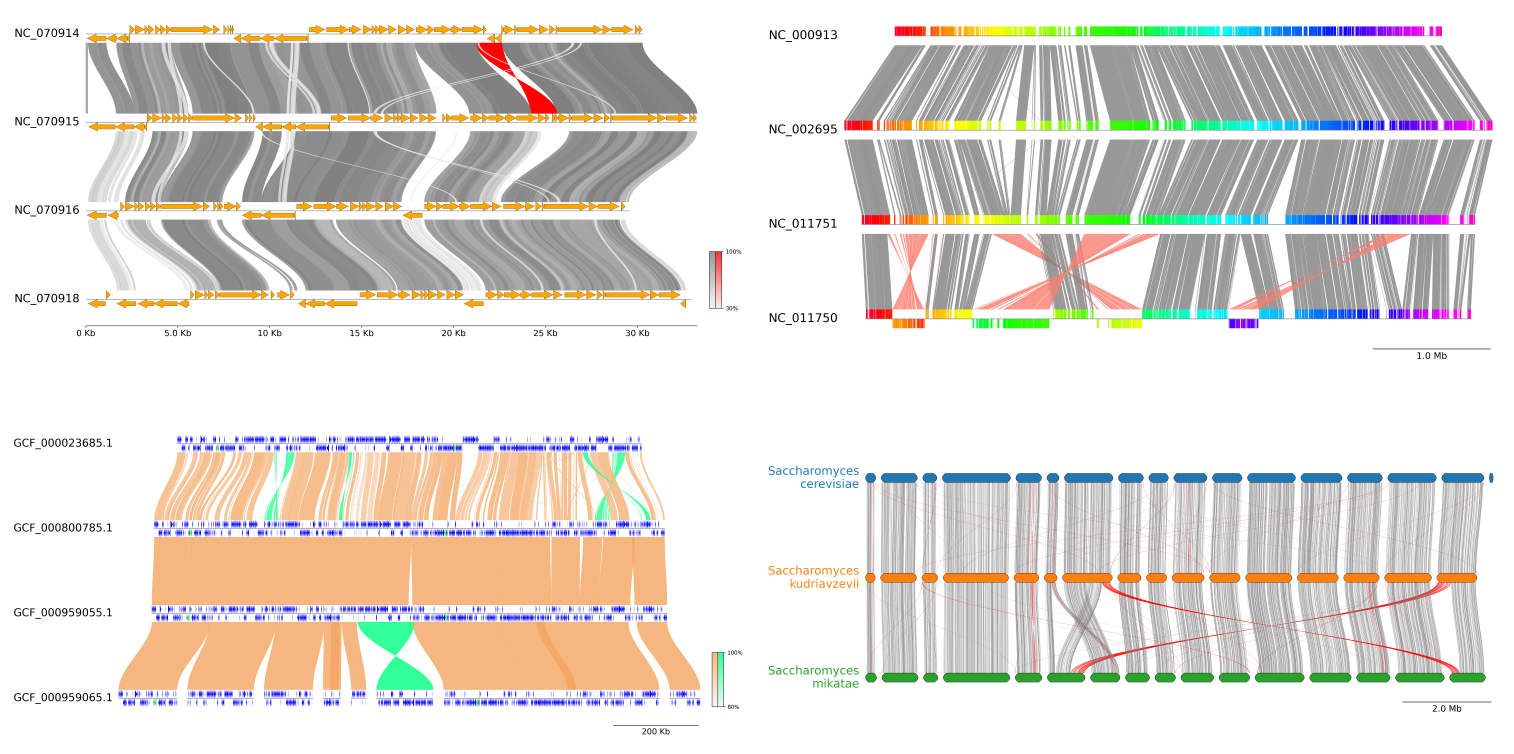
Fig.1 pyGenomeViz example plot gallery
✨ GUI (Web Application) functionality is newly added from v0.4.0
 Fig.2 pyGenomeViz web application example (Demo Page)
Python 3.8 or later is required for installation.
Install PyPI package:
pip install pygenomeviz
Install bioconda package:
conda install -c conda-forge -c bioconda pygenomeviz
Use Docker (Image Registry):
Case1. Run CLI Workflow:
docker run -it --rm ghcr.io/moshi4/pygenomeviz:latest pgv-mummer -h
Case2. Launch GUI (Web Application):
docker run -it --rm -p 8501:8501 ghcr.io/moshi4/pygenomeviz:latest pgv-gui
Jupyter notebooks containing code examples below is available here.
from pygenomeviz import GenomeViz

name, genome_size = "Tutorial 01", 5000
cds_list = ((100, 900, -1), (1100, 1300, 1), (1350, 1500, 1), (1520, 1700, 1), (1900, 2200, -1), (2500, 2700, 1), (2700, 2800, -1), (2850, 3000, -1), (3100, 3500, 1), (3600, 3800, -1), (3900, 4200, -1), (4300, 4700, -1), (4800, 4850, 1))

gv = GenomeViz()
track = gv.add_feature_track(name, genome_size)
for idx, cds in enumerate(cds_list, 1):
    start, end, strand = cds
    track.add_feature(start, end, strand, label=f"CDS{idx:02d}")

gv.savefig("example01.png")
from pygenomeviz import GenomeViz

genome_list = (
    {"name": "genome 01", "size": 1000, "cds_list": ((150, 300, 1), (500, 700, -1), (750, 950, 1))},
    {"name": "genome 02", "size": 1300, "cds_list": ((50, 200, 1), (350, 450, 1), (700, 900, -1), (950, 1150, -1))},
    {"name": "genome 03", "size": 1200, "cds_list": ((150, 300, 1), (350, 450, -1), (500, 700, -1), (700, 900, -1))},
)

gv = GenomeViz(tick_style="axis")
for genome in genome_list:
    name, size, cds_list = genome["name"], genome["size"], genome["cds_list"]
    track = gv.add_feature_track(name, size)
    for idx, cds in enumerate(cds_list, 1):
        start, end, strand = cds
        track.add_feature(start, end, strand, label=f"gene{idx:02d}", linewidth=1, labelrotation=0, labelvpos="top", labelhpos="center", labelha="center")

# Add links between "genome 01" and "genome 02"
gv.add_link(("genome 01", 150, 300), ("genome 02", 50, 200))
gv.add_link(("genome 01", 700, 500), ("genome 02", 900, 700))
gv.add_link(("genome 01", 750, 950), ("genome 02", 1150, 950))
# Add links between "genome 02" and "genome 03"
gv.add_link(("genome 02", 50, 200), ("genome 03", 150, 300), normal_color="skyblue", inverted_color="lime", curve=True)
gv.add_link(("genome 02", 350, 450), ("genome 03", 450, 350), normal_color="skyblue", inverted_color="lime", curve=True)
gv.add_link(("genome 02", 900, 700), ("genome 03", 700, 500), normal_color="skyblue", inverted_color="lime", curve=True)
gv.add_link(("genome 03", 900, 700), ("genome 02", 1150, 950), normal_color="skyblue", inverted_color="lime", curve=True)

gv.savefig("example02.png")
from pygenomeviz import GenomeViz

exon_regions1 = [(0, 210), (300, 480), (590, 800), (850, 1000), (1030, 1300)]
exon_regions2 = [(1500, 1710), (2000, 2480), (2590, 2800)]
exon_regions3 = [(3000, 3300), (3400, 3690), (3800, 4100), (4200, 4620)]

gv = GenomeViz()
track = gv.add_feature_track(name=f"Exon Features", size=5000)
track.add_exon_feature(exon_regions1, strand=1, plotstyle="box", label="box", labelrotation=0, labelha="center")
track.add_exon_feature(exon_regions2, strand=-1, plotstyle="arrow", label="arrow", labelrotation=0, labelha="center", facecolor="darkgrey", intron_patch_kws={"ec": "red"})

exon_labels = [f"exon{i+1}" for i in range(len(exon_regions3))]
track.add_exon_feature(exon_regions3, strand=1, plotstyle="bigarrow", label="bigarrow", facecolor="lime", linewidth=1, exon_labels=exon_labels, labelrotation=0, labelha="center", exon_label_kws={"y": 0, "va": "center", "color": "blue"})

gv.savefig("example03.png")
from pygenomeviz import Genbank, GenomeViz, load_example_dataset

gbk_files, _ = load_example_dataset("enterobacteria_phage")
gbk = Genbank(gbk_files[0])

gv = GenomeViz()
track = gv.add_feature_track(gbk.name, gbk.range_size)
track.add_genbank_features(gbk)

gv.savefig("example04.png")
from pygenomeviz import Gff, GenomeViz, load_example_gff

gff_file = load_example_gff("enterobacteria_phage.gff")
gff = Gff(gff_file, min_range=5000, max_range=25000)

gv = GenomeViz(fig_track_height=0.7, tick_track_ratio=0.5, tick_style="bar")
track = gv.add_feature_track(gff.name, size=gff.range_size, start_pos=gff.min_range)
track.add_gff_features(gff, plotstyle="arrow", facecolor="tomato")
track.set_sublabel()

gv.savefig("example05.png")
from pygenomeviz import Genbank, GenomeViz, load_example_dataset

gv = GenomeViz(
    fig_track_height=0.7,
    feature_track_ratio=0.2,
    tick_track_ratio=0.4,
    tick_style="bar",
    align_type="center",
)

gbk_files, links = load_example_dataset("escherichia_phage")
for gbk_file in gbk_files:
    gbk = Genbank(gbk_file)
    track = gv.add_feature_track(gbk.name, gbk.range_size)
    track.add_genbank_features(gbk, facecolor="limegreen", linewidth=0.5, arrow_shaft_ratio=1.0)

for link in links:
    link_data1 = (link.ref_name, link.ref_start, link.ref_end)
    link_data2 = (link.query_name, link.query_start, link.query_end)
    gv.add_link(link_data1, link_data2, v=link.identity, curve=True)

gv.savefig("example06.png")
Since pyGenomeViz is implemented based on matplotlib, users can easily customize the figure in the manner of matplotlib. Here are some tips for figure customization.
- Add
GC Content&GC skewsubtrack - Add annotation label & fillbox
- Add colorbar for links identity
Code
from pygenomeviz import Genbank, GenomeViz, load_example_dataset

gv = GenomeViz(
    fig_width=12,
    fig_track_height=0.7,
    feature_track_ratio=0.5,
    tick_track_ratio=0.3,
    tick_style="axis",
    tick_labelsize=10,
)

gbk_files, links = load_example_dataset("erwinia_phage")
gbk_list = [Genbank(gbk_file) for gbk_file in gbk_files]
for gbk in gbk_list:
    track = gv.add_feature_track(gbk.name, gbk.range_size, labelsize=15)
    track.add_genbank_features(gbk, plotstyle="arrow")

min_identity = int(min(link.identity for link in links))
for link in links:
    link_data1 = (link.ref_name, link.ref_start, link.ref_end)
    link_data2 = (link.query_name, link.query_start, link.query_end)
    gv.add_link(link_data1, link_data2, v=link.identity, vmin=min_identity)

# Add subtracks to top track for plotting 'GC content' & 'GC skew'
gv.top_track.add_subtrack(ratio=0.7, name="gc_content")
gv.top_track.add_subtrack(ratio=0.7, name="gc_skew")

fig = gv.plotfig()

# Add label annotation to top track
top_track = gv.top_track  # or, gv.get_track("MT939486") or gv.get_tracks()[0]
label, start, end = "Inverted", 310000 + top_track.offset, 358000 + top_track.offset
center = int((start + end) / 2)
top_track.ax.hlines(1.5, start, end, colors="red", linewidth=1, linestyles="dashed", clip_on=False)
top_track.ax.text(center, 2.0, label, fontsize=12, color="red", ha="center", va="bottom")

# Add fillbox to top track
x, y = (start, start, end, end), (1, -1, -1, 1)
top_track.ax.fill(x, y, fc="lime", linewidth=0, alpha=0.1, zorder=-10)

# Plot GC content for top track
pos_list, gc_content_list = gbk_list[0].calc_gc_content()
pos_list += gv.top_track.offset  # Offset is required if align_type is not 'left'
gc_content_ax = gv.top_track.subtracks[0].ax
gc_content_ax.set_ylim(bottom=0, top=max(gc_content_list))
gc_content_ax.fill_between(pos_list, gc_content_list, alpha=0.2, color="blue")
gc_content_ax.text(gv.top_track.offset, max(gc_content_list) / 2, "GC(%) ", ha="right", va="center", color="blue")

# Plot GC skew for top track
pos_list, gc_skew_list = gbk_list[0].calc_gc_skew()
pos_list += gv.top_track.offset  # Offset is required if align_type is not 'left'
gc_skew_abs_max = max(abs(gc_skew_list))
gc_skew_ax = gv.top_track.subtracks[1].ax
gc_skew_ax.set_ylim(bottom=-gc_skew_abs_max, top=gc_skew_abs_max)
gc_skew_ax.fill_between(pos_list, gc_skew_list, alpha=0.2, color="red")
gc_skew_ax.text(gv.top_track.offset, 0, "GC skew ", ha="right", va="center", color="red")

# Set coloarbar for link
gv.set_colorbar(fig, vmin=min_identity)

fig.savefig("example07.png")
- Add legends
- Add colorbar for links identity
Code
from matplotlib.lines import Line2D
from matplotlib.patches import Patch

from pygenomeviz import Genbank, GenomeViz, load_example_dataset

gv = GenomeViz(
    fig_width=10,
    fig_track_height=0.5,
    feature_track_ratio=0.5,
    tick_track_ratio=0.3,
    align_type="center",
    tick_style="bar",
    tick_labelsize=10,
)

gbk_files, links = load_example_dataset("enterobacteria_phage")
for idx, gbk_file in enumerate(gbk_files):
    gbk = Genbank(gbk_file)
    track = gv.add_feature_track(gbk.name, gbk.range_size, labelsize=10)
    track.add_genbank_features(
        gbk,
        label_type="product" if idx == 0 else None,  # Labeling only top track
        label_handle_func=lambda s: "" if s.startswith("hypothetical") else s,  # Ignore 'hypothetical ~~~' label
        labelsize=8,
        labelvpos="top",
        facecolor="skyblue",
        linewidth=0.5,
    )

normal_color, inverted_color, alpha = "chocolate", "limegreen", 0.5
min_identity = int(min(link.identity for link in links))
for link in links:
    link_data1 = (link.ref_name, link.ref_start, link.ref_end)
    link_data2 = (link.query_name, link.query_start, link.query_end)
    gv.add_link(link_data1, link_data2, normal_color, inverted_color, alpha, v=link.identity, vmin=min_identity, curve=True)

fig = gv.plotfig()

# Add Legends (Maybe there is a better way)
handles = [
    Line2D([], [], marker=">", color="skyblue", label="CDS", ms=10, ls="none"),
    Patch(color=normal_color, label="Normal Link"),
    Patch(color=inverted_color, label="Inverted Link"),
]
fig.legend(handles=handles, bbox_to_anchor=(1, 1))

# Set colorbar for link
gv.set_colorbar(fig, bar_colors=[normal_color, inverted_color], alpha=alpha, vmin=min_identity, bar_label="Identity", bar_labelsize=10)

fig.savefig("example08.png")
pyGenomeViz provides CLI workflow for visualization of genome alignment or
reciprocal best-hit CDS search results with MUMmer or MMseqs or progressiveMauve.
Each CLI workflow requires the installation of additional dependent tools to run.
See pgv-mummer document for details.
Download example dataset: pgv-download-dataset -n erwinia_phage
⚠️ MUMmer must be installed in advance to run
pgv-mummer --gbk_resources MT939486.gbk MT939487.gbk MT939488.gbk LT960552.gbk \
           -o mummer_example --tick_style axis --align_type left --feature_plotstyle arrow

See pgv-mmseqs document for details.
Download example dataset: pgv-download-dataset -n enterobacteria_phage
⚠️ MMseqs must be installed in advance to run
pgv-mmseqs --gbk_resources NC_019724.gbk NC_024783.gbk NC_016566.gbk NC_013600.gbk NC_031081.gbk NC_028901.gbk \
           -o mmseqs_example --fig_track_height 0.7 --feature_linewidth 0.3 --tick_style bar --curve \
           --normal_link_color chocolate --inverted_link_color limegreen --feature_color skyblue

See pgv-pmauve document for details.
Download example dataset: pgv-download-dataset -n escherichia_coli
⚠️ progressiveMauve must be installed in advance to run
pgv-pmauve --seq_files NC_000913.gbk NC_002695.gbk NC_011751.gbk NC_011750.gbk \
           -o pmauve_example --tick_style bar

pyGenomeViz implements GUI (Web Application) functionality using streamlit as an option (Demo Page). Users can easily visualize the genome data of Genbank files and their comparison results with GUI. See pgv-gui document for details.
pyGenomeViz implements HTML file output functionality for interactive data visualization.
In API, HTML file can be output using savefig_html method. In CLI, user can select HTML file output option.
As shown below, data tooltip display, pan/zoom, object color change, text change, etc are available in HTML viewer
(Demo Page).
pyGenomeViz was inspired by
pyGenomeViz is a python package designed for linear genome visualization. If you are interested in circular genome visualization, check out my other python package pyCirclize.
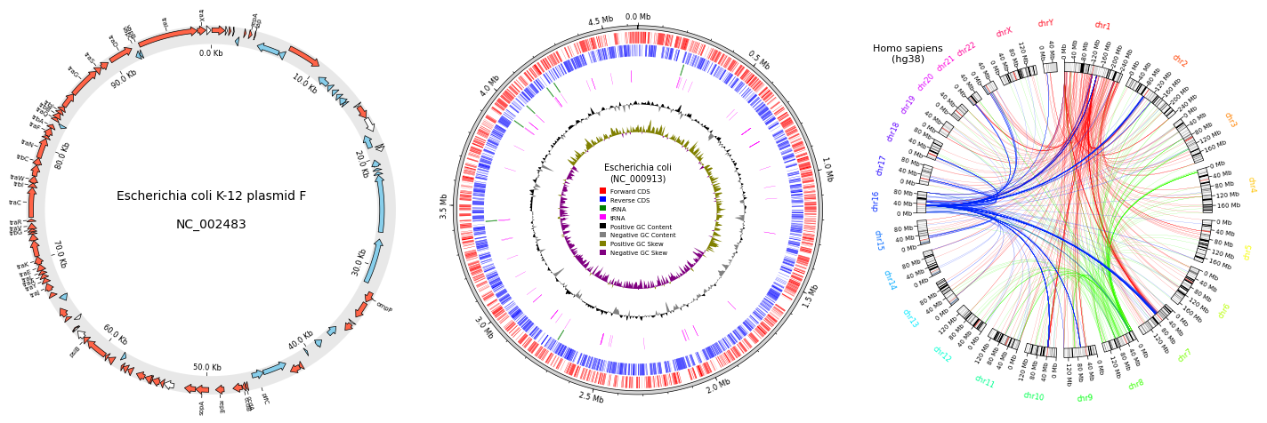
Fig. pyCirclize example plot gallery