Lattice Boltzmann Fluid Simulation

Using Intel MPI for inter-process communication and OpenMP 4.5 for parallel GPU execution.

Timings for graphs were taken on BlueCrystal Phase 4 with the following configs

CPU - Intel Xeon E5-2680 v4
GPU - Nvidia Tesla P100

Parallel CPU

Scatter and Gather
MPI_Scatter and MPI_Gather to decompose the domain by rows
Reduce
MPI_Reduce for tree reductions of data across processes
Neighbourhood Collective
Cartesian communicators and MPI_Neighbor_alltoall for halo exchange
Async Halo Exchange
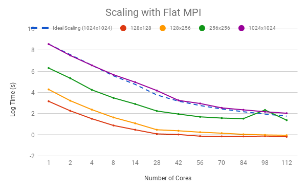
MPI_Ineighbor_alltoall allows asynchronous halo exchanges. The caveat with this is that the inner computations is O(N^2) whereas the halo exchange is O(N) so this only becomes useful on the larger problems with many cores where there is some balance between these factors due to communication overhead. It means that the CPU is not kept idle if there is a network bottleneck.

Time on multiple CPU cores across different problem grid sizes

Parallel GPU

OpenMP 4.5 pragmas produce CUDA code

#pragma omp target update to()

to transfer data to the GPU and

#pragma omp target update from()

to transfer data from the GPU.
Although these are very expensive operations and must be used sparingly.

#pragma omp target teams distribute parallel for reduction(+:tot_u) collapse(2)

offloads work to the GPU to be executed in parallel.

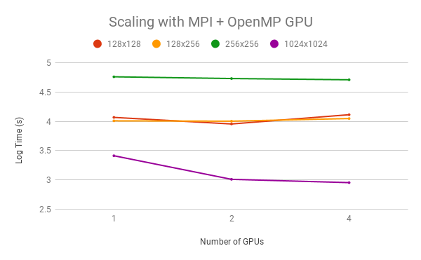
Time on multiple GPUs across different problem grid sizes

Compiling and running

To compile type make. Editing the values for CC and CFLAGS in the Makefile can be used to enable different compiler options or use a different compiler. These can also be passed on the command line:

$ make CFLAGS="-O3 -fopenmp -DDEBUG"

Input parameter and obstacle files are all specified on the command line of the d2q9-bgk executable.

Usage:

$ ./d2q9-bgk <paramfile> <obstaclefile>

eg:

$ ./d2q9-bgk input_256x256.params obstacles_256x256.dat

Checking results

An automated result checking function is provided that requires you to load a particular Python module (module load languages/anaconda2). Running make check will check the output file (average velocities and final state) against some reference results. By default, it should look something like this:

$ make check
python check/check.py --ref-av-vels-file=check/128x128.av_vels.dat --ref-final-state-file=check/128x128.final_state.dat --av-vels-file=./av_vels.dat --final-state-file=./final_state.dat
Total difference in av_vels : 5.270812566515E-11
Biggest difference (at step 1219) : 1.000241556248E-14
  1.595203170657E-02 vs. 1.595203170658E-02 = 6.3e-11%

Total difference in final_state : 5.962977334129E-11
Biggest difference (at coord (6,2)) : 1.000588500943E-14
  3.329122639178E-02 vs. 3.329122639179E-02 = 3e-11%

Both tests passed!

This script takes both the reference results and the results to check (both average velocities and final state). This is also specified in the makefile and can be changed like the other options:

$ make check REF_AV_VELS_FILE=check/128x256.av_vels.dat REF_FINAL_STATE_FILE=check/128x256.final_state.dat
python check/check.py --ref-av-vels-file=check/128x256.av_vels.dat --ref-final-state-file=check/128x256.final_state.dat --av-vels-file=./av_vels.dat --final-state-file=./final_state.dat
...

All the options for this script can be examined by passing the --help flag to it.

$ python check/check.py --help
usage: check.py [-h] [--tolerance TOLERANCE] --ref-av-vels-file
                REF_AV_VELS_FILE --ref-final-state-file REF_FINAL_STATE_FILE
...

Visualisation

You can view the final state of the simulation by creating a .png image file using a provided Gnuplot script: