| Object Detections | Ground truth Scene Graph | Generated Scene Graph |
|---|---|---|
 |
 |
 |
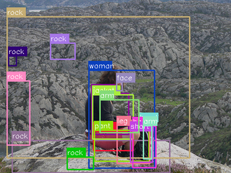
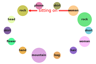
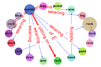
In this visualization, woman sitting on rock is a zero-shot triplet, which means that the combination of woman, sitting on and rock has never been observed during training. However, each of the object and predicate has been observed, but together with other objects and predicate. For example, woman sitting on chair has been observed and is not a zero-shot triplet. Making correct predictions for zero-shots is very challenging, so in our papers [1,2] we address this problem and improve zero-shot as well as few-shot results. See examples of zero-shots in the Visual Genome (VG) dataset at Zero_Shot_VG.ipynb.
This repository accompanies two papers:
See the code for my another ICCV 2021 paper Context-aware Scene Graph Generation with Seq2Seq Transformers at https://github.com/layer6ai-labs/SGG-Seq2Seq.
The code in this repo is based on the amazing code for Neural Motifs by Rowan Zellers. Our code uses torchvision.models.detection, so can be run in PyTorch 1.2 or later.
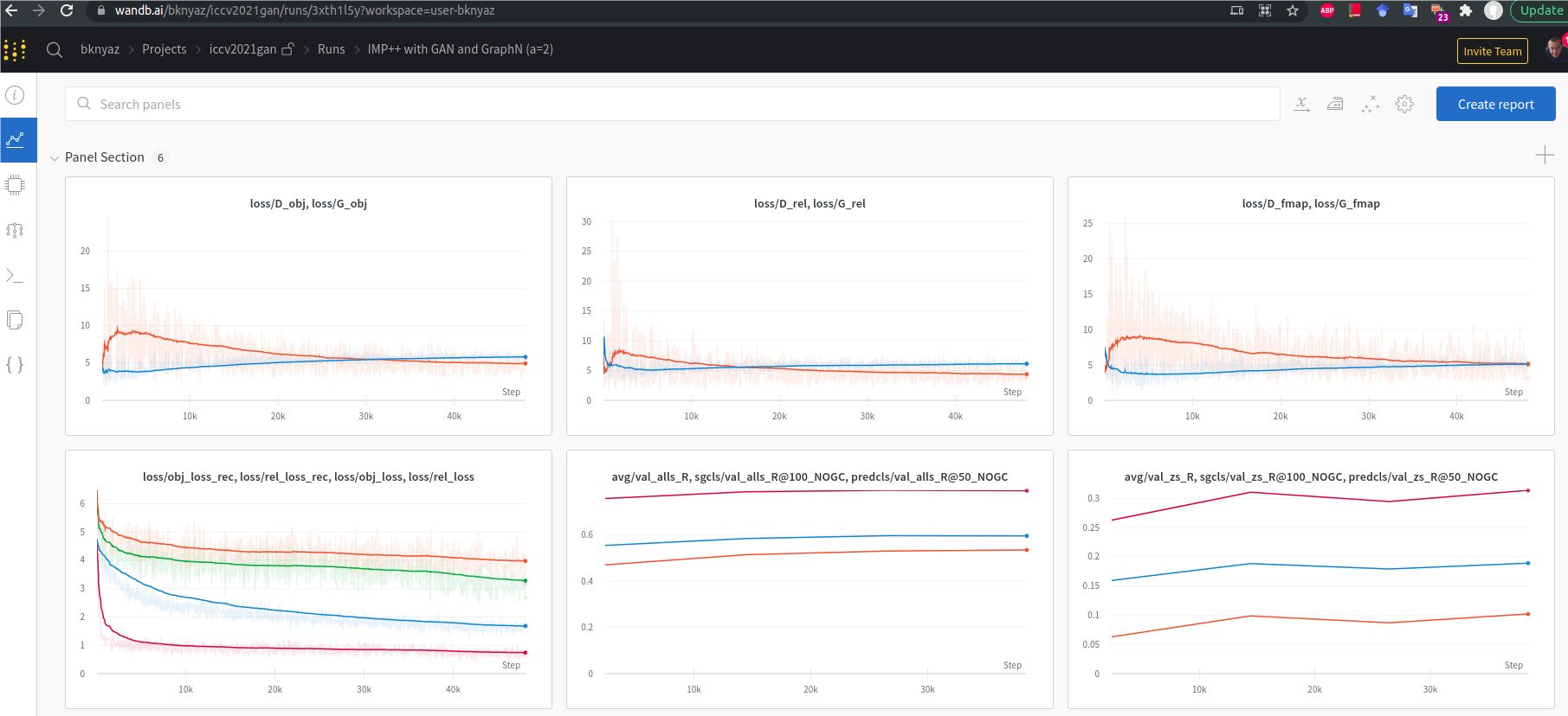
Weights and Biases is a cool tool to track your machine learning experiments that I used in this project. It is free (in most cases) and very user-friendly, which is very helpful for complex projects with lots of metrics (like SGG).
See our Weights and Biases (W & B) project for the results on different SGG metrics and training curves.
- Python >= 3.6
- PyTorch >= 1.2
- Other standard Python libraries
Should be enough to install these libraries (in addition to PyTorch):
conda install -c anaconda h5py cython dill pandas
conda install -c conda-forge pycocotools tqdm
Results in our papers [1,2] were obtained on a single GPU 1080Ti/2080Ti/RTX6000 with 11-24GB of GPU memory and 32GB of RAM. MultiGPU training is unfortunately not supported in this repo.
To use the edge feature model from Rowan Zellers' model implementations (default argument -edge_model motifs in our code), it is necessary to build the following function:
cd lib/draw_rectangles; python setup.py build_ext --inplace; cd ../..;
Visual Genome or GQA data will be automatically downloaded after the first call of python main.py -data $data_path. After downloading, the script will generate the following directories (make sure you have at least 60GB of disk space in $data_path):
data_path
│   VG
│   │   VG.tar
│   │   VG_100K (this will appear after extracting VG.tar)
│   │   ...
│
└───GQA # optional
│   │   GQA_scenegraphs.tar
│   │   sceneGraphs (this will appear after extracting GQA_scenegraphs.tar)
|   |   ...
If downloading fails, you can download manually using the links from lib/download.py. Alternatively, the VG can be downloaded following Rowan Zellers' instructions, while GQA can be downloaded from the GQA official website.
To train SGG models on VG, download Rowan Zellers' VGG16 detector checkpoint and save it as ./data/VG/vg-faster-rcnn.tar.
To train our GAN models from [2], it is necessary to first extract and save real object features from the training set of VG by running:
python extract_features.py -data ./data/ -ckpt ./data/VG/vg-faster-rcnn.tar -save_dir ./data/VG/
The script will generate ./data/VG/features.hdf5 of around 30GB.
Our improved edge loss from [1] can be added to any SGG model that predicts edge labels rel_dists, which is a float valued tensor of shape (M,R), where R is the total number of predicate classes (e.g. 51 in Visual Genome). M is the total number of edges in a batch of scene graphs, including the background edges (edges without any semantic relationships).
The baseline loss used in most SGG works simply computes the cross-entropy between rel_dists and ground truth edge labels rel_labels (an integer tensor of length M):
baseline_edge_loss = torch.nn.functional.cross_entropy(rel_dists, rel_labels)
Our improved edge loss takes into account the extreme imbalance between the foreground and background edge terms. Foreground edges are those that have semantic ground truth annotations (e.g. on, has, wearing, etc.). In datasets like Visual Genome, scene graph annotations are extremely sparse, i.e. the number of foreground edges (M_FG) is significantly lower than the total number of edges M.
baseline_edge_loss = torch.nn.functional.cross_entropy(rel_dists, rel_labels)
M = len(rel_labels)
M_FG = torch.sum(rel_labels > 0)
our_edge_loss = baseline_edge_loss * M / M_FG
Our improved loss significantly improves all SGG metrics, in particular zero and few shots. See [1] for the results and discussion why our loss works well.
See the full code of different losses in lib/losses.py.
In this example I provide the pseudo code for adding the GAN model to a given SGG model. See the full code in main.py.
from torch.nn.functional import cross_entropy as CE

# Assume the SGG model (sgg_model) returns features for
# nodes (nodes_real) and edges (edges_real) as well as global features (fmap_real).

# 1. Main SGG model object and relationship classification losses (L_CLS)

obj_dists, rel_dists = sgg_model.predict(nodes_real, edges_real)  # predict node and edge labels
node_loss = CE(obj_dists, gt_objects)
M = len(rel_labels)
M_FG = torch.sum(rel_labels > 0)
our_edge_loss = CE(rel_dists, rel_labels) *  M / M_FG  # use our improved edge loss from [1]

L_CLS = node_loss + our_edge_loss  # SGG total loss from [1]
L_CLS.backward()
F_optimizer.step()  # update the sgg_model (main SGG model F)

# 2. GAN-based updates

# Scene Graph perturbations (optional)
gt_objects_fake = sgp.perturb(gt_objects, gt_rels)  # we only perturb nodes (object labels)

# Generate global feature maps using our GAN conditioned on (perturbed) scene graphs
fmap_fake = gan(gt_objects_fake, gt_boxes, gt_rels)

# Extract node and edge features from fmap_fake
nodes_fake, edges_fake = sgg_model.node_edge_features(fmap_fake)

# Make SGG predictions for the node and edge features
# Detach the gradients to avoid bad collaboration of G and F
obj_dists_fake, rel_dists_fake = sgg_model.predict(nodes_fake.detach(),
                                                   edges_fake.detach())

# 2.1. Generator (G) losses

# Adversarial losses
L_ADV_G_nodes = gan.loss(nodes_fake, labels_fake=gt_objects_fake)
L_ADV_G_edges = gan.loss(edges_fake, labels_fake=rel_labels)
L_ADV_G_global = gan.loss(fmap_fake)

# Reconstruction losses
L_REC_nodes = CE(obj_dists_fake, gt_objects_fake)
L_REC_edges = CE(rel_dists_fake, rel_labels) *  M / M_FG  # use our improved edge loss from [1]

# Total G loss
loss_G_F = L_ADV_G_nodes + L_ADV_G_edges + L_ADV_G_global + L_REC_nodes + L_REC_edges
loss_G_F.backward()
F_optimizer.step()  # update the sgg_model (main SGG model F)
G_optimizer.step()  # update the generator (G) of the GAN

# 2.1. Discriminator (D) losses

# Adversarial losses
L_ADV_D_nodes = gan.loss(node_real, nodes_fake, labels_fake=gt_objects_fake, labels_real=gt_objects)
L_ADV_D_edges = gan.loss(edge_real, edges_fake, labels_fake=rel_labels, labels_real=rel_labels)
L_ADV_D_global = gan.loss(fmap_real, fmap_fake)

# Total D loss
loss_D = L_ADV_D_nodes + L_ADV_D_edges + L_ADV_D_global
loss_D.backward()  # update the discriminator (D) of the GAN
D_optimizer.step()
Adding our GAN also consistently improves all SGG metrics. See [2] for the results, model description and analysis.
Results of R@100 are reported below obtained using Faster R-CNN with VGG16 as a backbone. No graph constraint evaluation is used. For graph constraint results and other details, see the W&B project.
| Model | Paper | Checkpoint | W & B | Zero-Shots | 10-shots | 100-shots | All-shots |
|---|---|---|---|---|---|---|---|
| IMP+1 | IMP / Neural Motifs | link | link | 8.7 | 19.2 | 38.4 | 47.8 |
| IMP++2 | our BMVC 2020 | link | link | 8.8 | 21.6 | 40.6 | 48.7 |
| IMP++ with GAN3 | our ICCV 2021 | link | link | 9.3 | 22.2 | 41.5 | 50.0 |
| IMP++ with GAN and GraphN scene graph perturbations4 | our ICCV 2021 | link | link | 10.2 | 21.7 | 40.9 | 49.8 |
-
1:
python main.py -data ./data -ckpt ./data/vg-faster-rcnn.tar -save_dir ./results/IMP_baseline -loss baseline -b 24 -
2:
python main.py -data ./data -ckpt ./data/vg-faster-rcnn.tar -save_dir ./results/IMP_dnorm -loss dnorm -b 24 -
3:
python main.py -data ./data -ckpt ./data/vg-faster-rcnn.tar -save_dir ./results/IMP_GAN -loss dnorm -b 24 -gan -largeD -vis_cond ./data/VG/features.hdf5 -
4:
python main.py -data ./data -ckpt ./data/vg-faster-rcnn.tar -save_dir ./results/IMP_GAN_graphn -loss dnorm -b 24 -gan -largeD -vis_cond ./data/VG/features.hdf5 -perturb graphn -L 0.2 -topk 5 -graphn_a 2-
-graphn_a 5: checkpoint, W & B project -
-graphn_a 10: checkpoint, W & B project -
-graphn_a 20: checkpoint, W & B project
-
Evaluation on the VG test set will be run at the end of the training script. To re-run evaluation: python main.py -data ./data -ckpt ./results/IMP_GAN_graphn/vgrel.pth -pred_weight $x, where $x is the weight for rare predicate classes, which is 1 for default, but can be increased to improve certain metrics like mean recall (see the Appendix in our paper [2] for more details).
To inspect the features generated with GANs, it is necessary to first extract and save node/edge/global features. This can be done similarly to the code in extract_features.py, but replacing the real features with the ones produced by the GAN.
See this jupyter notebook to inspect generated feature quality.
See this jupyter notebook to inspect scene graph perturbation methods.
Please follow the details in our papers to obtain SGGen/SGDet results, which are based on using the original Neural Motifs code.
Pull-requests to add training and evaluation SGGen/SGDet models with the VGG16 or another backbone are welcome.
Note: these instructions are for our BMVC 2020 paper [1] and have not been tested in the last version of the repo
To train an SGCls/PredCls model with our loss on GQA: python main.py -data ./data -loss dnorm -split gqa -lr 0.002 -save_dir ./results/GQA_sgcls # takes about 1 day. Or download our GQA-SGCls-1 checkpoint
In the trained checkpoints of this repo I used a slightly different edge model in UnionBoxesAndFeats -edge_model raw_boxes. To use Neural Motifs's edge model, use flag -edge_model motifs (default in the current version of the repo).
Follow these steps to train and evaluate an SGGen model on GQA:
-
Fine-tune Mask R-CNN on GQA:
python pretrain_detector.py gqa ./data ./results/pretrain_GQA# takes about 1 day. Or download our GQA-detector checkpoint -
Train SGCls:
python main.py -data ./data -lr 0.002 -split gqa -nosave -loss dnorm -ckpt ./results/pretrain_GQA/gqa_maskrcnn_res50fpn.pth -save_dir ./results/GQA_sgdet# takes about 1 day. Or download our GQA-SGCls-2 checkpoint. This checkpoint is different from SGCls-1, because here the model is trained on the features of the GQA-pretrained detector. This checkpoint can be used in the next step. -
Evaluate SGGen:
python main.py -data ./data -split gqa -ckpt ./results/GQA_sgdet/vgrel.pth -m sgdet -nosave -nepoch 0# takes a couple hours
See an example of detecting objects and obtaining scene graphs for GQA test images at Scene_Graph_Predictions_GQA.ipynb.
Please use these references to cite our papers or code:
@inproceedings{knyazev2020graphdensity,
  title={Graph Density-Aware Losses for Novel Compositions in Scene Graph Generation},
  author={Knyazev, Boris and de Vries, Harm and Cangea, Cătălina and Taylor, Graham W and Courville, Aaron and Belilovsky, Eugene},
  booktitle={British Machine Vision Conference (BMVC)},
  pdf={http://arxiv.org/abs/2005.08230},
  year={2020}
}
@inproceedings{knyazev2020generative,
  title={Generative Compositional Augmentations for Scene Graph Prediction},
  author={Boris Knyazev and Harm de Vries and Cătălina Cangea and Graham W. Taylor and Aaron Courville and Eugene Belilovsky},
  booktitle={International Conference on Computer Vision (ICCV)},
  pdf={https://arxiv.org/abs/2007.05756},
  year={2021}
}
