blt2589/FlowPy

Flow-Py

Flow-Py is an open source tool to compute gravitational mass flows (GMF) run out and intensity. The main objective is to compute the spatial extent of GMF, which consists of the starting, transit and runout zones of GMF on the surface of a three dimensional terrain. The resulting run out is mainly dependent on the terrain and the location of the starting/release point. No time-dependent equations are solved in the model. Flow-Py uses existing statistical-data-based approaches for solving the routing and stopping of GMF.

The tool has been designed to be computationally light, allowing the application on a regional scale including a large number of GMF paths. The Flow-Py code is written in python and takes advantage of pythons object oriented class structure. The well structured model implementation allows users to address specific GMF research questions by keeping the parameterization flexible and the ability to include custom model extensions and add-ons.

Setting up Python3 environment

Flow-Py works on Linux and Windows operating systems in a Python3 environment.

Linux, Windows

run the following command in the terminal to install the required packages:

pip install -r requirements.txt

If you have trouble installing GDAL or rasterio on Windows use these links to get the required version directly from their website, first install GDAL and then rasterio.

GDAL: https://www.lfd.uci.edu/~gohlke/pythonlibs/#gdal

rasterio: https://www.lfd.uci.edu/~gohlke/pythonlibs/#rasterio

MacOS

Flow-Py has not been tested it on MacOS. If you are able to run it there, please give us feedback.

Running the Code

Once the required libraries are installed the model runs via the main.py script. Flow-Py can be started in the terminal or with a simple GUI which helps to organize the input data and parameterizations.

Graphical user interface version

python3 main.py --gui 

Terminal version

The terminal version runs with the following arguments:

• alpha_angle (controls the run out angle induced stopping and routing)
• exponent (controls concentration of routing flux and therefore the lateral spread)
• working directory path
• path to DEM raster (.tiff or .asc)
• path to release raster (.tiff or .asc)
• (Optional) flux threshold (positive number) flux_threshold=xx (limits spreading with the exponent)
• (Optional) Max Z^δ (positive number) max_z_delta=xx (max kinetic energy height, turbulent friction)

python3 main.py alpha_angle exponent working_directory path_to_dem path_to_release flux_threshold=positiv_number(Optional) max_z_delta=positiv_number(Optional

Here is an example for running Flow-Py on a simple parabolic slope with a channelized path and a small dam between the transit and run out area. Input data can be found in the example directory.

Example:

python3 main.py 25 8 ./examples/dam/ ./examples/dam/dam_010m_standard_cr100_sw250_f2500.20.6_n0.asc ./examples/dam/release_dam.tif flux=0.003 max_z=270

Input Files

All raster files (DEM, release, ...) must be in the .asc or .tif format.

All rasters need the same resolution (normal sizes are e.g. 5x5 or 10x10 meters).

All Layers need the same spatial extend, with no data values < 0 (standard no data values = -9999).

The locations identified as release areas need values > 0. (see release.tif in examples)

Output

All outputs are in the .tiff raster format in the same resolution and extent as the input raster layers.

• z_delta: the maximum z_delta of all paths for every raster cell (geometric measure of process magnitude, can be associated to kinetic energy/velocity)
• Flux: The maximum routing flux of all paths for every raster cell
• sum_z_delta: z_delta summed up over all paths on every raster cell
• Cell_Counts: number of paths that route flux through a raster cell
• Flow Path Travel Angle, FP_TA: the gamma angle along the flow path
• Straight Line Travel Angle, SL_TA: Saves the gamma angle, while the distances are calculated via a straight line from the release cell to the current cell

Back-tracking extension

The back-tracking extension is an example of a custom built model extension used to identify the release areas, paths and deposition areas of GMF directly endangering infrastructure.

To activate the back-tracking extension an additional raster layer describing the spatial extent of the infrastructure must be called by the model. The GUI version of the model has a field where an infrastructure layer can be inserted. For the terminal version the “infra= path_to_infrastructure_raster” must be included as an additional argument (see command below).

python3 main.py alpha_angle exponent working_directory path_to_dem path_to_release infra=path_to_infrastructure(Optional) flux_threshold=positiv_number(Optional) max_z_delta=positiv_number(Optional)

Example:

python3 main.py 25 8 ./examples/dam/ ./examples/dam/dam_010m_standard_cr100_sw250_f2500.20.6_n0.asc ./examples/dam/release_dam.tif infra=./examples/dam/infra.tif flux=0.003 max_z=270

The infrastructure layer must be in the same extent and resolution as the other input layers (DEM and release raster). Raster cells that contain infrastructure must have values > zero, raster cells with values = 0 represent locations without infrastructure (see infrastructure.tif in example folder). Different integers can be used to differentiate types of infrastructure, where higher valued infrastructure should correspond to higher integers . When a raster cell is associated with endangering infrastructure the integer associated with the infrastructure type is saved in the back-tracking output layer. When a raster cell is associated with endangering more than one type of infrastructure the larger integer is saved to the back tracking output.

Back-tracking output:

• z_delta: the maximum z_delta of all paths for every raster cell (geometric measure of process magnitude, can be associated to kinetic energy/velocity)
• Flux: The maximum routing flux of all paths for every raster cell
• Flow Path Travel Angle, FP_TA: the gamma angle along the flow path
• Straight Line Travel Angle, SL_TA: Saves the travel angle along a straight line, i.e. distances are calculated via a direct line from the release cell to the current cell
• Back-tracking: Areas identified as endangering infrastructure.

Motivation

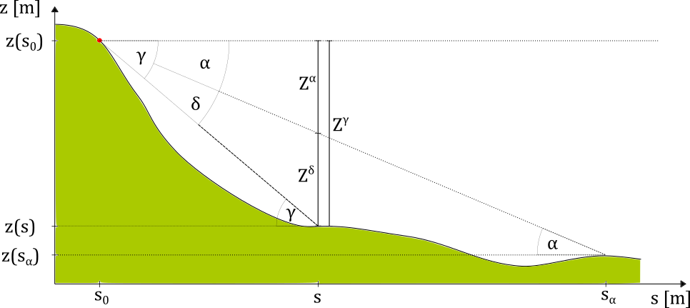
Fig. 1: Definition of angles and geometric measures for the calculation of Z^δ, where s is the projected distance along the path and z(s) the corresponding altitude.

The model equations that determine the run out in three dimensional terrain are mainly motivated with respect to simple, geometric, two dimensional concepts [0,3,4] in conjunction with ideas existing algorithms for flow routing in three dimensional terrain [1,2], controlling the main routing and final stopping of the flow.

Figure 1 summarizes the basic concept of a constant run out angle (alpha) with the corresponding geometric relations in two dimensions along a possible process path.

The local travel angle gamma is defined by the altitude difference and projected distance along the path, from the release point to the current location.

The angle delta is the difference between the local travel angle gamma and the runout angle alpha and is related to Z^δ, so when delta equals zero or gamma equals alpha, the maximum runout distance is reached.

Z^α can be interpreted as dissipation energy.

Z^γ is the altitude difference between the starting point and the current calculation step at the projected distance s.

Z^δ is the difference between Z^γ and Z^α, so when Z^δ is lower or equal zero the stopping criterion is met and the flow stops. Z^δ is associated to the process magnitude and can be interpreted as the kinetic energy or velocity of the process.

The major drawback of implementing the geometric runout angle concepts is that they require a predefined flow path in two dimensional terrain. To allow for an enhanced routing in three dimensional terrain without prior knowledge of the flow path we combine these concepts [4] with extensions of existing algorithms [1,2,3] that are described in the following sections.

Spatial Input and Iterative Calculation Steps on the Path

In nature a GMF has one or more release areas that span over single or multiple release cells. Flow-Py computes the so called path, which is defined as the spatial extent of the routing from each release cell. Each release area (single raster cell in release area layer) has it's own unique path (collection of raster cells), and a location on the terrain (a single raster cell) can belong to many paths. Flow-Py identifies the path with spatial iterations starting with a release area raster cell and only iterating over cells which receive routing flux. The corresponding functions are implemented in the code in the flow_class.calc_distribution() function.

To route on the surface of the three dimensional terrain, operating on a quadrilateral grid, we implement the geometric concepts that have been sketched in the model motivation utilizing the following cell definitions:

​

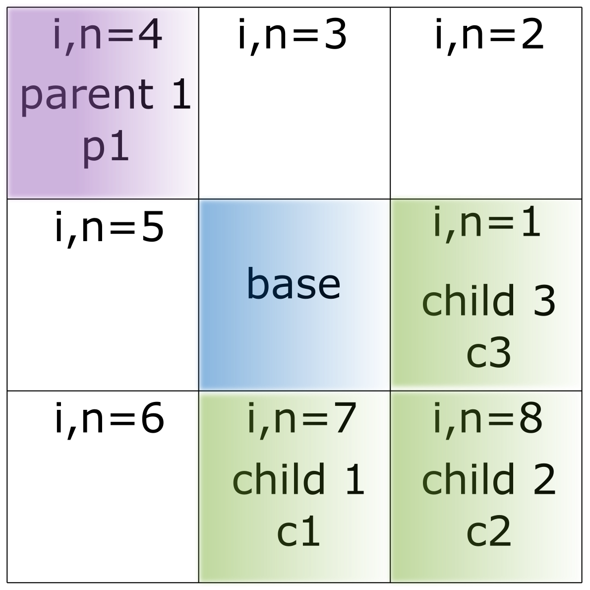
Fig. 2: Definition of parent, base, child and neighbors, as well as the indexing around the base.

Each path calculation starts with a release cell and operates on the raster, requiring the definition of parent, base, child and neighbor cells (see Fig. 2). The base cell is the cell being calculated on the current spatial iteration step. The 8 raster cells surrounding the base cell are called neighbor cells (n, i) which have the potential to be parents (supplying flux to base cell), or a child (receive flux from the base cell). In 2d the base cell corresponds to the cell/location at the distance s along the path in Fig. 1.

Every base has at least one parent cell, except in the first calculation step from the release cell, where we start our calculation, this would be at s = s₀ in Fig. 1.

During an iteration step a raster cell from the iteration list is identified as the current base cell. The routing flux is calculated across the base cell from the parent cell to possible child cells. The goal is to keep the spatial iteration steps to a minimum, which is achieved by only adding neighbor cells to the iteration list that have flux routed to them from the base cell and do not meet either of the stopping conditions. These cells are called child cells. Child cells that are not already on the iteration list are added to the list and flow_class python object is created for the raster cell. The child cells flow_class has the parent added to it as a source for routing flux. By being added to the iteration list the cell has been recognized as being part of the GMF path and will be the base cell for a future iteration step.

When the iteration list is empty and all potential children fulfill one of the stopping criteria:

• Z^δ has to be smaller than zero: Z^δ < 0,
• Routing Flux has to be smaller than the flux cut off: R_i < R_Stop,

the path calculation is finished. The required information is saved from the cell class to the summarizing output raster files. Then the calculation starts again for the next release cell and respective flow path. The spatial extent and magnitude for all release cells are summarized in the output raster files, which represent the overlay of all paths.

Every path is independent from the other, but depending on the information we want to extract, we save the highest values (e.g. Z^δ) or sums (e.g.Cell Counts) of different paths to the output raster file.

Z^δ

For each base cell in a path we solve the equations (6,7 and 8) for every neighbor n, if Z_bn^δ is higher than zero, this neighbor is defined as a potential child of this base, and routing in this direction is possible.

Here S_bn is the projected distance between the base and the neighbor.

As Z_bn^δ can be interpreted as process magnitude (and kinetic energy or velocity respectively) it is possible to limit this value to a maximum. In comparison to process based modeling approaches this would correspond to maximum velocity induced by a velocity dependent turbulent friction term.

The projected path lengths, or total travel distance to one of the neighbors (S_n) equals the path length to the base (S_b) plus the path from base to the neighbor (S_bn), which reads:

As there are many possibilities for the path from the starting point to the actual cell or base, the shortest path is taken into account, corresponding to the highest Z^δ in the base. If Z^δ_max is set to infinity, or as in the code to 8848 m (= Mount Everest), we can calculate the shortest path from the starting point to the base and yields the total projected travel distance:

This equations determine the routing and corresponding run out distance for the process, the next steps demonstrate how spreading is handled on the surface of the three dimensional terrain.

Persistence based routing

The persistence contribution P_i aims to reproduce the behavior of inertia, and takes the change in flow direction into account [3]. The direction contribution is scaled with the process magnitude Z^δ_parent, such that the direction from a parent cell with higher process magnitude has more effect on the path routing and direction.

The direction contributions D_n are defined by the cosine of the angle between parent, base and child/neighbor minus pi:

Therefore the direction contribution limits the maximum number of potential children to three, getting input via the persistence function from one parent.

In the first calculation step, at the release or start cell no parent cells are defined and the persistence is set to one. So the first calculation step is solely determined by the terrain contribution.

Terrain based routing

The terrain based routing is solely dependent on the slope angle phi. The exponent exp allows to control the divergence of the spreading. The Holmgren (1994) algorithm [1] is used in different kind of models and works well for avalanches but also rockfall or soil slides. For avalanches an exponent of 8 shows good results. To reach a single flow in step terrain (rockfall, soil slides, steepest descend), an exponent of 75 is considered.

Holmgrem Algorithm from 1994 [1]

To overcome the challenge of routing in flat or uphill terrain, we adapted the slope angle phi for the normalized terrain contribution to:

Routing Flux

The routing flux summarizes the persistence and terrain contributions according to Eq.(16):

where i is the direction and n are the neighbors from 1 to 8. R_i is then the routing flux in direction i. R_b is the flux in the base, for a release cell or starting cell the flux of the base equals one. The result of Eq. (16) is a 3 x 3 array with assigned flux values. A normalization stage is then required to bring the sum of the R_i's to the value of R_b. This aims at avoiding loss of flux [2].

Flow Chart / Overview

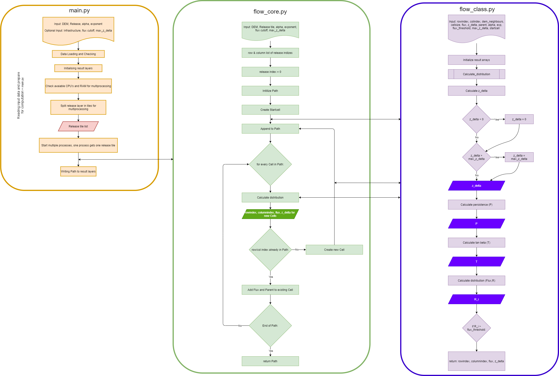
In Fig. 3 the algorithm of the computational implementation is sketched, including function and files names with respect to the code in the repository.

The file main.py handles the input for the computation and splits the release layer in tiles and saves them in a release list. Then the main.py starts one process per tile, which calls the flow_core.py and starts the calculation for one release cell and the corresponding path. The number of processes is depending on the hardware setting (CPU and RAM). Whenever a new cell is created flow_core.py calls flow_class.py and makes a new instance of this class, which is saved in the path. When the calculation in flow_core.py is finished it returns the path to main.py which saves the result to the output rasters.

Fig.3: Flow chart of the Flow-Py computational process and an overview of the files and what they manage.

References

[0] [Heim, A. (1932).]: Bergstürze und Menschenleben

[1] Holmgren, P. (1994). Multiple flow direction algorithms for runoff modelling in grid based elevation models: an empirical evaluation. Hydrological Processes, 8:327–334.

[2] Horton, P., Jaboyedoff, M., Rudaz, B., and Zimmermann, M. (2013). Flow-R, a model for susceptibility mapping of debris flows and other gravitational hazards at a regional scale. Natural Hazards and Earth System Science, 13:869–885.

[3] Gamma, P. (1999). dfwalk - Ein Murgang-Simulationsprogramm zur Gefahrenzonierung. PhD thesis, Universität Bern.

[4] [Huber, A., Fischer, J. T., Kofler, A., and Kleemayr, K. (2016).] Using spatially distributed statistical models for avalanche runout estimation. In International Snow Science Workshop, Breckenridge, Colorado, USA - 2016.

Contact and acknowledgment

For Questions contact:
Michael Neuhauser, Austrian Research Centre for Forest: Michael.Neuhauser@bfw.gv.at
Christopher D'Amboise, Austrian Research Centre for Forest: Christopher.DAmboise@bfw.gv.at

This study was carried out in the framework of the GreenRisk4Alps project ASP635, funded by the European Regional Development Fund through the Interreg Alpine Space programme. Additional financial support from the AvaRange (www.AvaRange.org, international cooperation project “AvaRange - Particle Tracking in Snow Avalanches” supported by the German Research Foundation (DFG) and the Austrian Science Fund (FWF, project number I 4274-N29) and the AvaFrame (www.AvaFrame.org, AvaFrame - The open Avalanche Framework is a cooperation between the Austrian Research Centre for Forests (Bundesforschungszentrum für Wald; BFW) and Austrian Avalanche and Torrent Service (Wildbach- und Lawinenverbauung; WLV) in conjunction with the Federal Ministry Republic of Austria: Agriculture, Regions and Tourism (BMLRT)) projects are greatly acknowledged.

Citation:

Michael Neuhauser, Christopher D'Amboise, Michaela Teich, Andreas Kofler, Andreas Huber, Reinhard Fromm, & Jan Thomas Fischer. (2021, June 24). Flow-Py: routing and stopping of gravitational mass flows (Version 1.0). Zenodo. http://doi.org/10.5281/zenodo.5027275