Diego Valle-Jones November 22, 2017
| Author: | Diego Valle-Jones |
| License: | BSD_3 |
| Status: | |
| Website: | https://hoyodesmog.diegovalle.net/aire.zmvm.html |
Tools for downloading pollution data for the Mexico City metro area. It can download real-time, daily maximum, minimum, or hourly average data for each of the pollution measuring stations or geographical zones in the Zona Metropolitana del Valle de México (greater Mexico City). It also includes the locations of all the measuring stations and a function to perform inverse distance weighting modified to work with wind direction.
You can always install the development version from GitHub:
if (!require(devtools)) {
    install.packages("devtools")
}
devtools::install_github('diegovalle/aire.zmvm')
To install the most recent package version from CRAN type:
install.packages("aire.zmvm")
library(aire.zmvm)
Note that the version on CRAN might not reflect the most recent changes made to this package.
The package consists mainly of four functions:
get_station_datato download data for each of the pollution (and wind and temperature) measuring stations.get_zone_datato download data for each of the 5 geographic zones of Mexico Cityget_latest_datato download the latest values for each of the pollution measuring stations.idw360Inverse distance weighting modified to work with degrees
library("aire.zmvm")
library("dplyr")
library("ggplot2")
library("ggseas")

o3 <- get_station_data(criterion = "MAXIMOS", # Can be one of MAXIMOS (daily maximum),
                                                # MINIMOS (daily minimum),
                                                # or HORARIOS (hourly average)
                       pollutant = "O3", # Can be one of "SO2", "CO", "NOX", "NO2", "NO", "O3",
                                         # "PM10", "PM25", "WSP", "WDR", "TMP", "RH"
                       year = 2009:2017) # A numeric vector, the earliest year allowed is 1986
knitr::kable(head(o3))| date | station_code | pollutant | unit | value |
|---|---|---|---|---|
| 2009-01-01 | ACO | O3 | ppb | 67 |
| 2009-01-02 | ACO | O3 | ppb | 71 |
| 2009-01-03 | ACO | O3 | ppb | 112 |
| 2009-01-04 | ACO | O3 | ppb | 91 |
| 2009-01-05 | ACO | O3 | ppb | 70 |
| 2009-01-06 | ACO | O3 | ppb | 71 |
# Daily max among all base stations
o3_max <- o3 %>%
  group_by(date) %>%
  summarise(max = ifelse(all(is.na(value)),
                         NA,
                         base::max(value, na.rm = TRUE))) %>%
  na.omit()

# ozone values at which a contingencia ambiental was declared
# and the dates during which they were valid
# source: http://www.aire.cdmx.gob.mx/descargas/ultima-hora/calidad-aire/pcaa/pcaa-modificaciones.pdf
contingencia <- data.frame(ppb = c(216, 210, 205, 199, 185, 155, 155),
  start = c(2009, 2009.4973, 2010.4973, 2011.5795,  2012.6052,  2016.291, 2016.4986),
  end = c(2009.4973, 2010.4945, 2011.4945, 2012.6025,   2016.2883, 2016.4959, Inf))
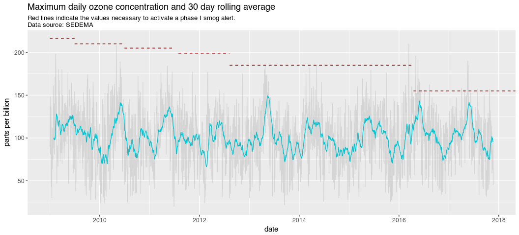
max_daily_df <- tsdf(ts(o3_max$max, start = c(2009,1), frequency = 365.25))
ggplot(max_daily_df,
       aes(x = x, y = y)) +
  geom_line(colour = "grey75", alpha = .5) +
  stat_rollapplyr(width = 30, align = "right", color = "#01C5D2") +
  #geom_vline(xintercept = 2015 + 183/365) +
  geom_segment(data = contingencia,
               aes(x=start, y=ppb, xend=end, yend=ppb), color="darkred", linetype = 2)  +
  xlab("date") +
  ylab("parts per billion") +
  ggtitle("Maximum daily ozone concentration and 30 day rolling average",
          subtitle = "Red lines indicate the values necessary to activate a phase I smog alert. \nData source: SEDEMA")
#> Warning: Removed 29 rows containing missing values (geom_path).