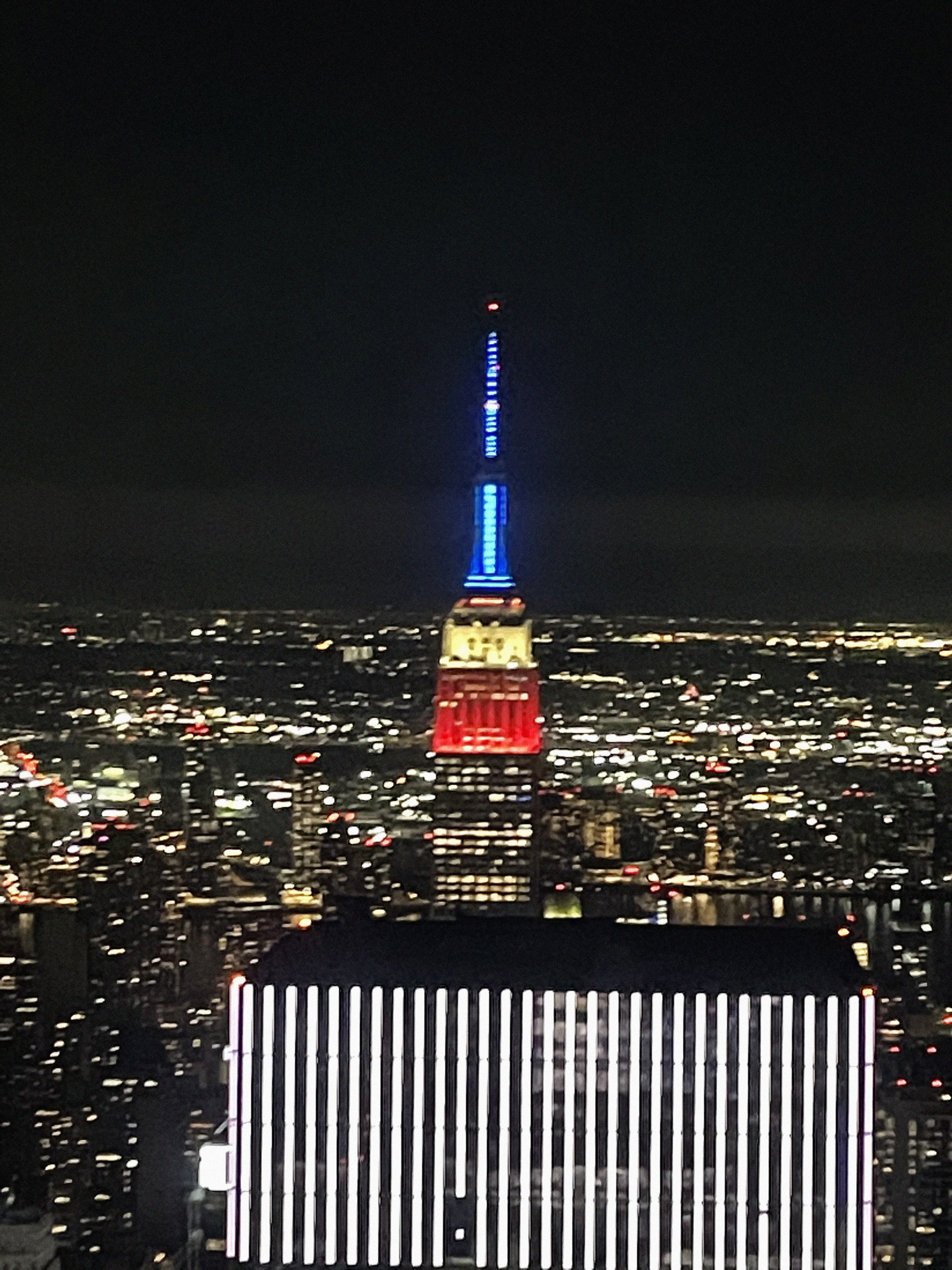
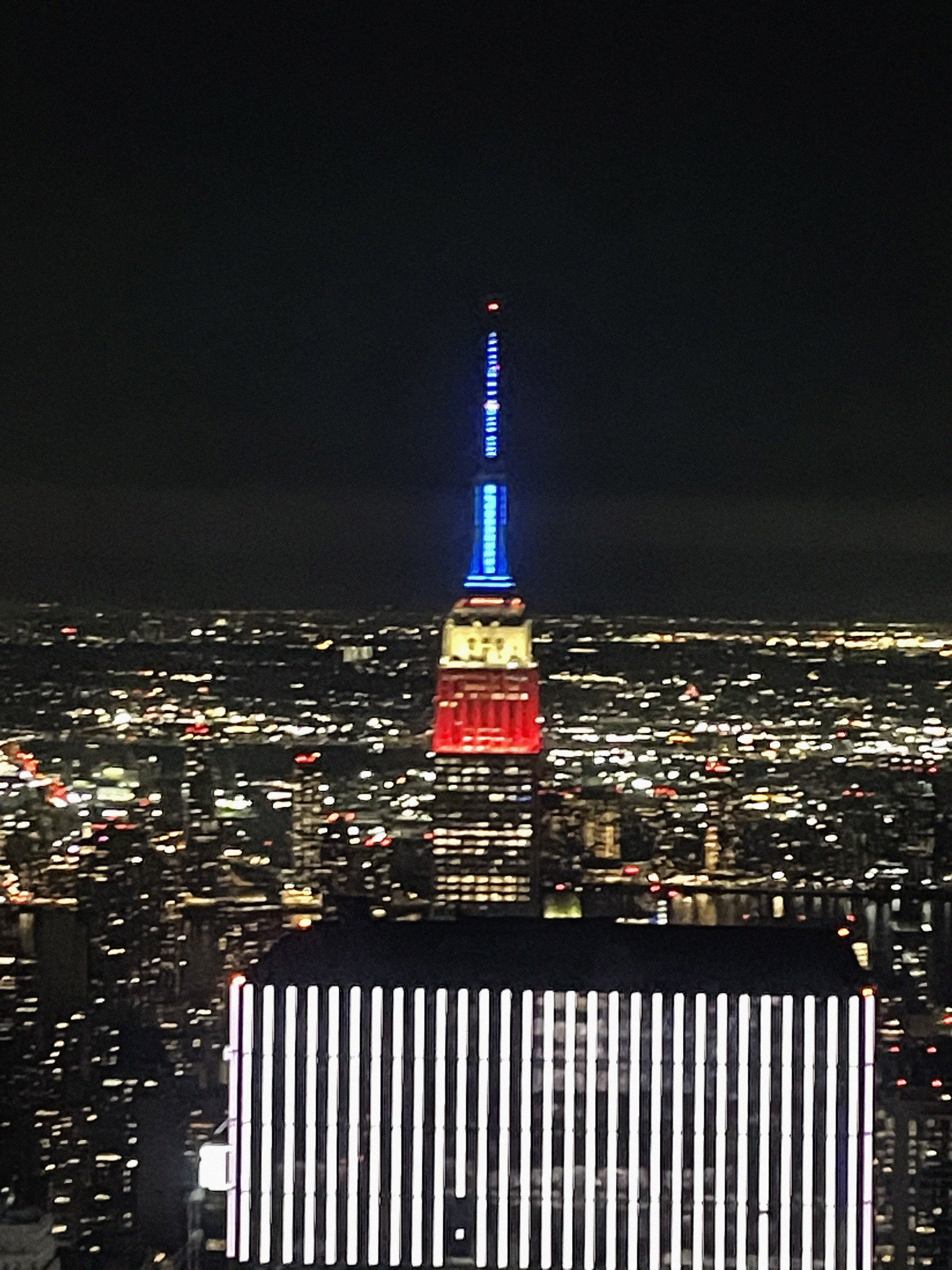
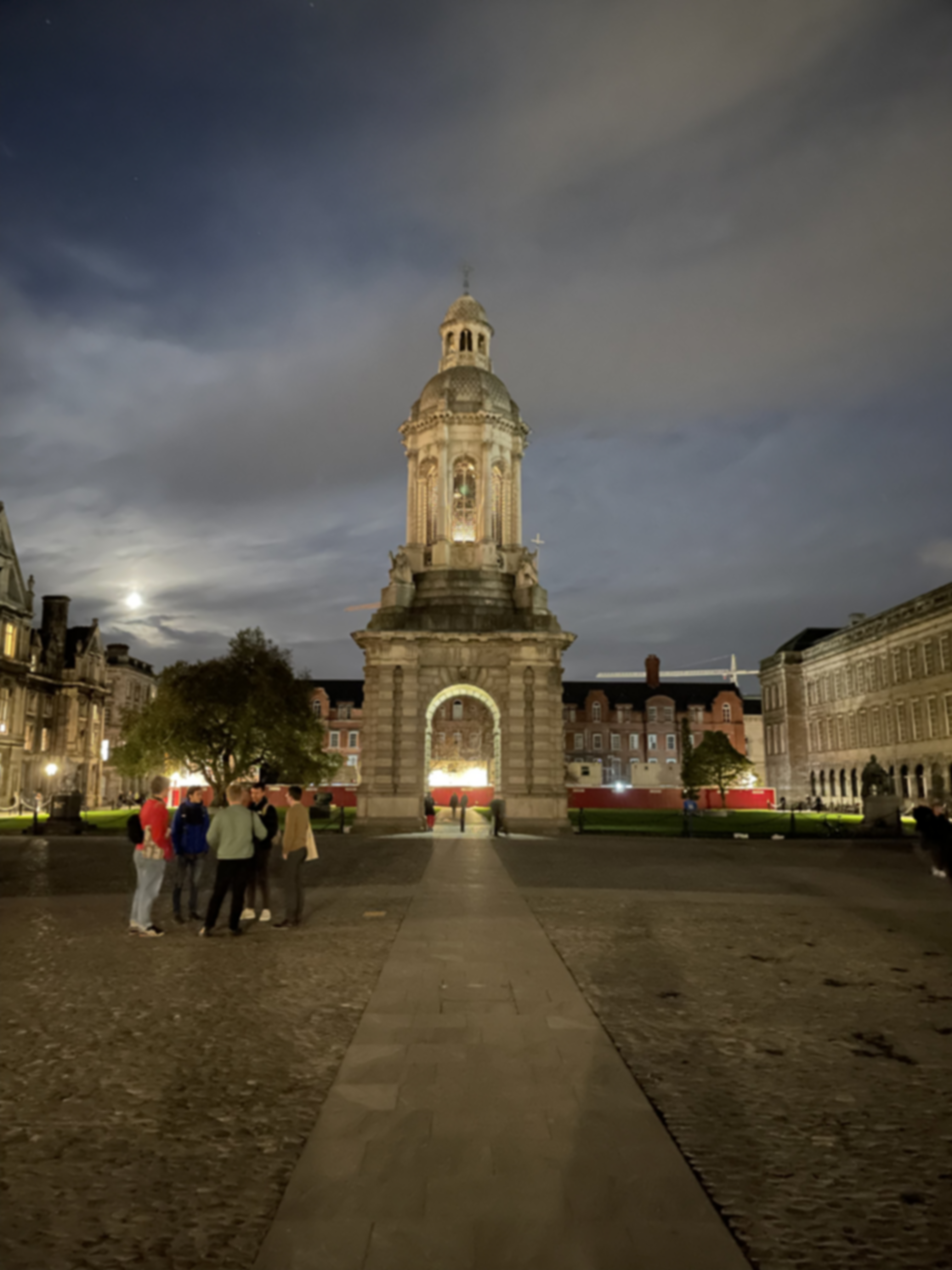
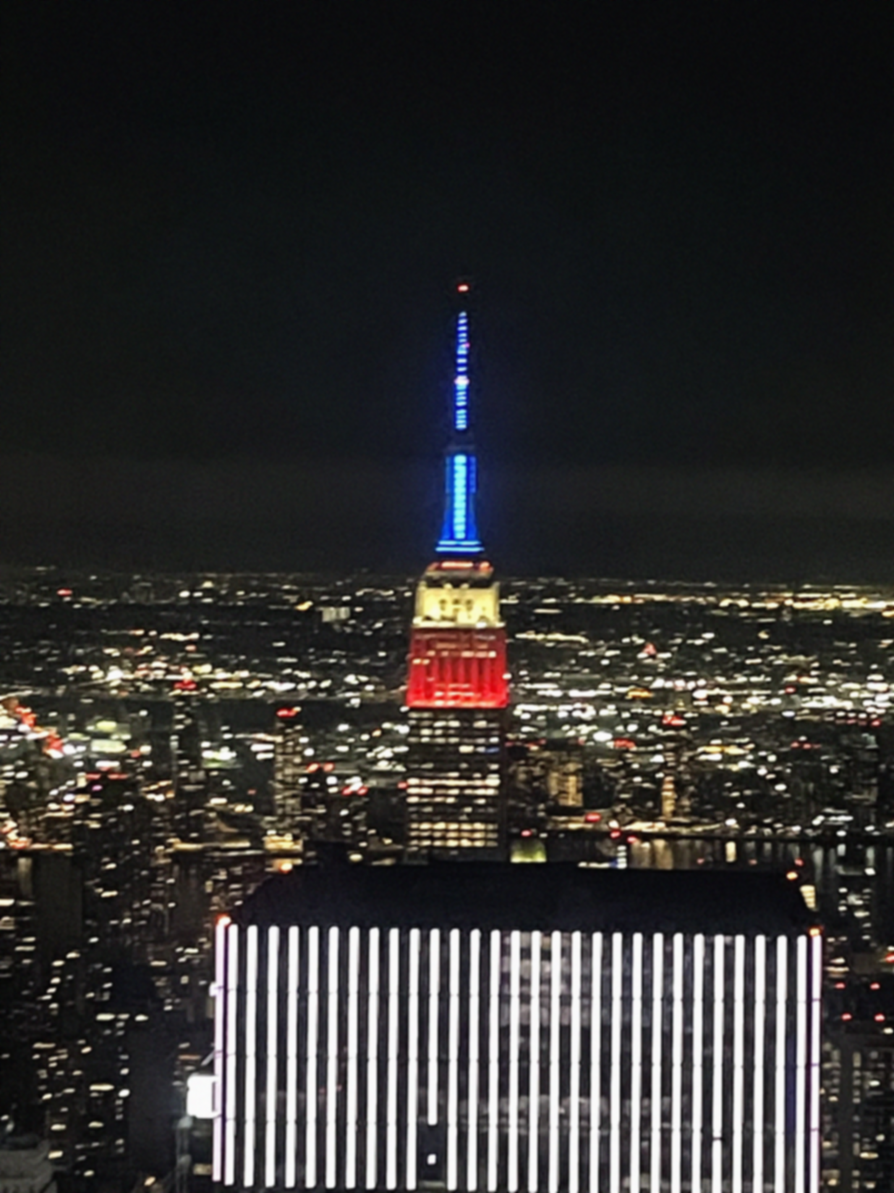
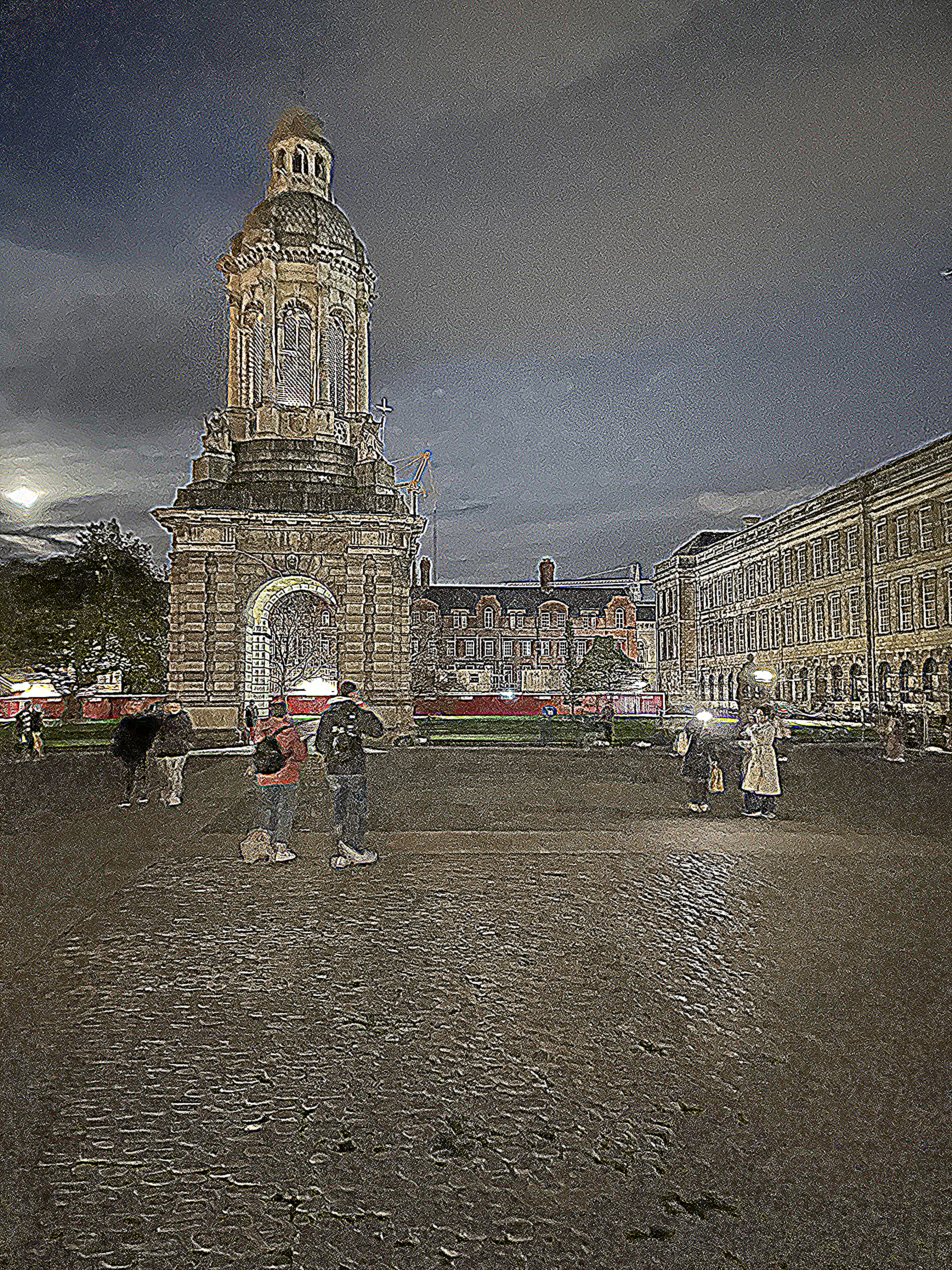
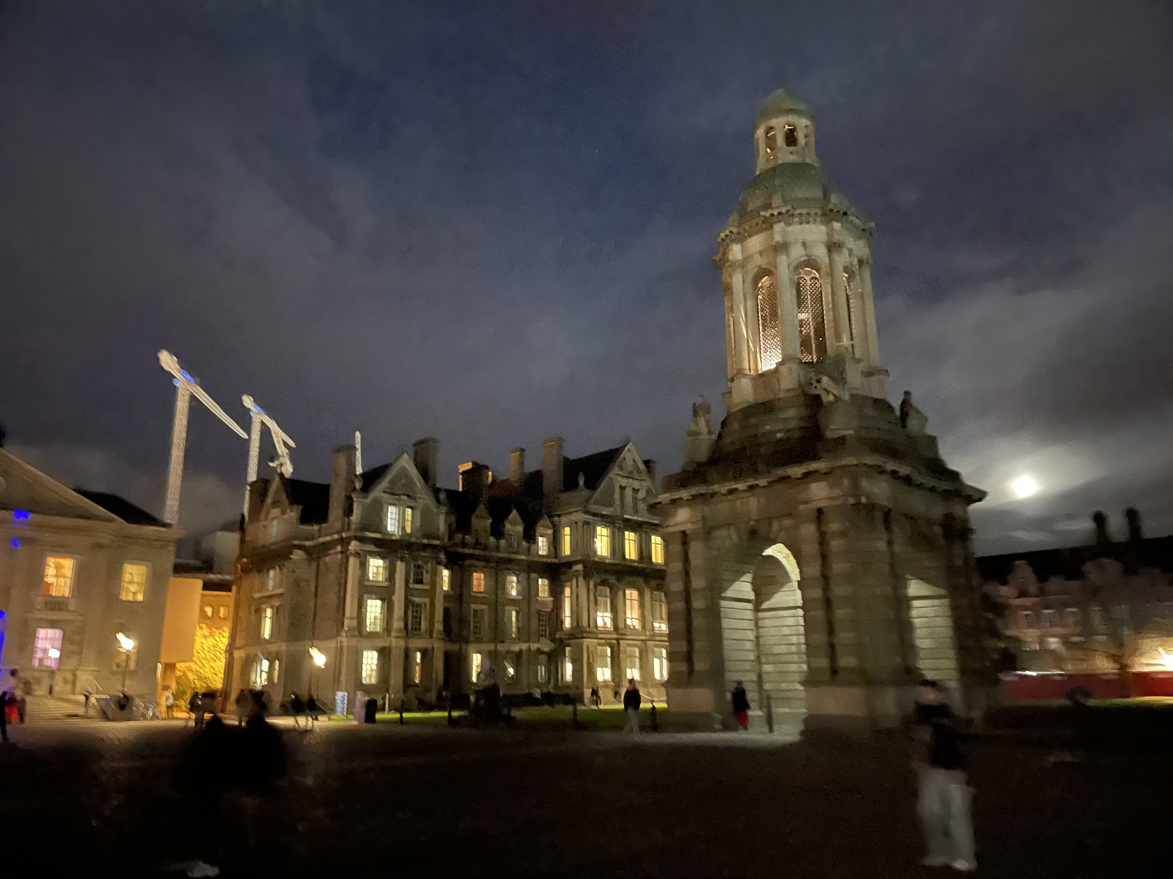
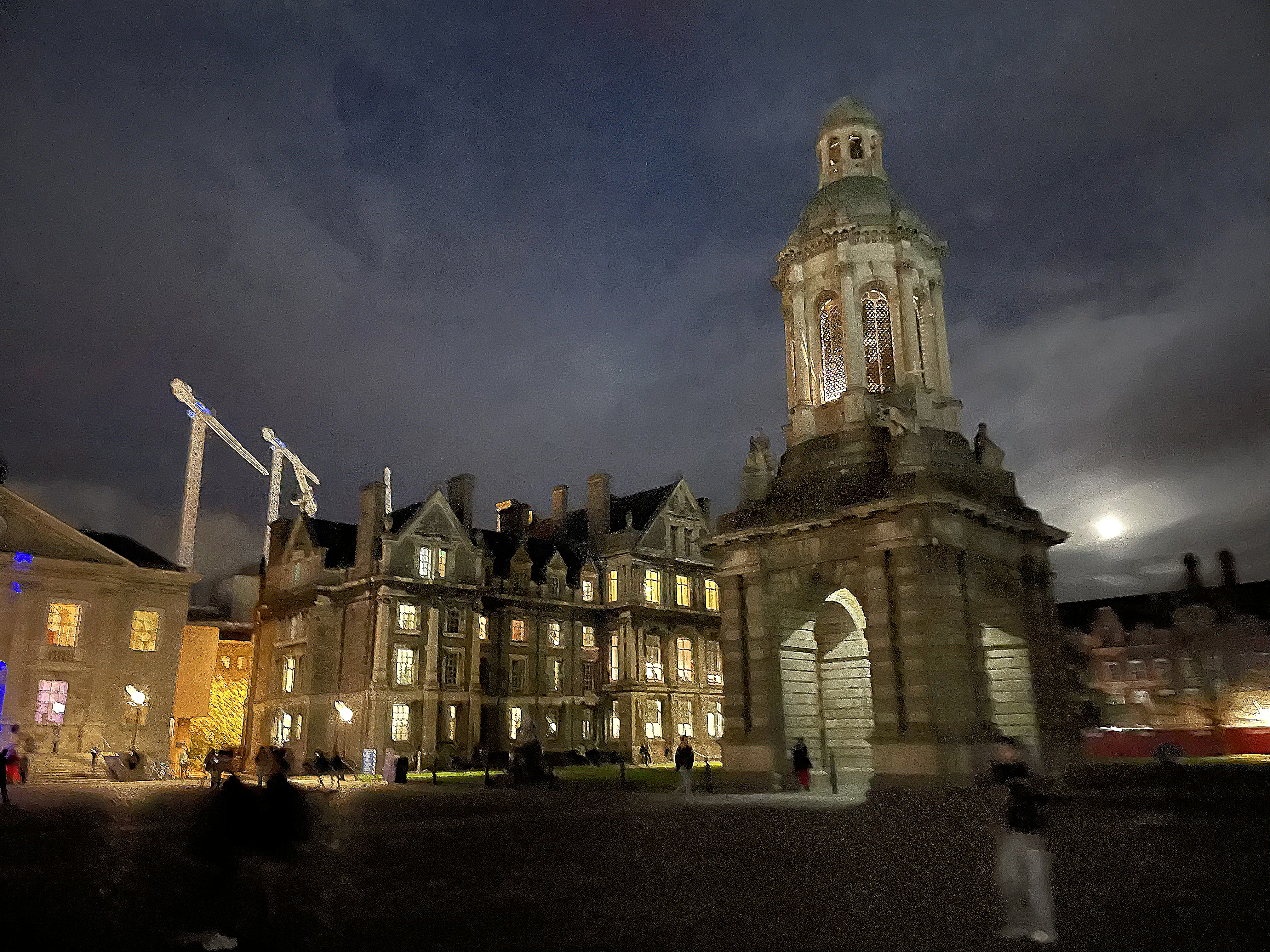
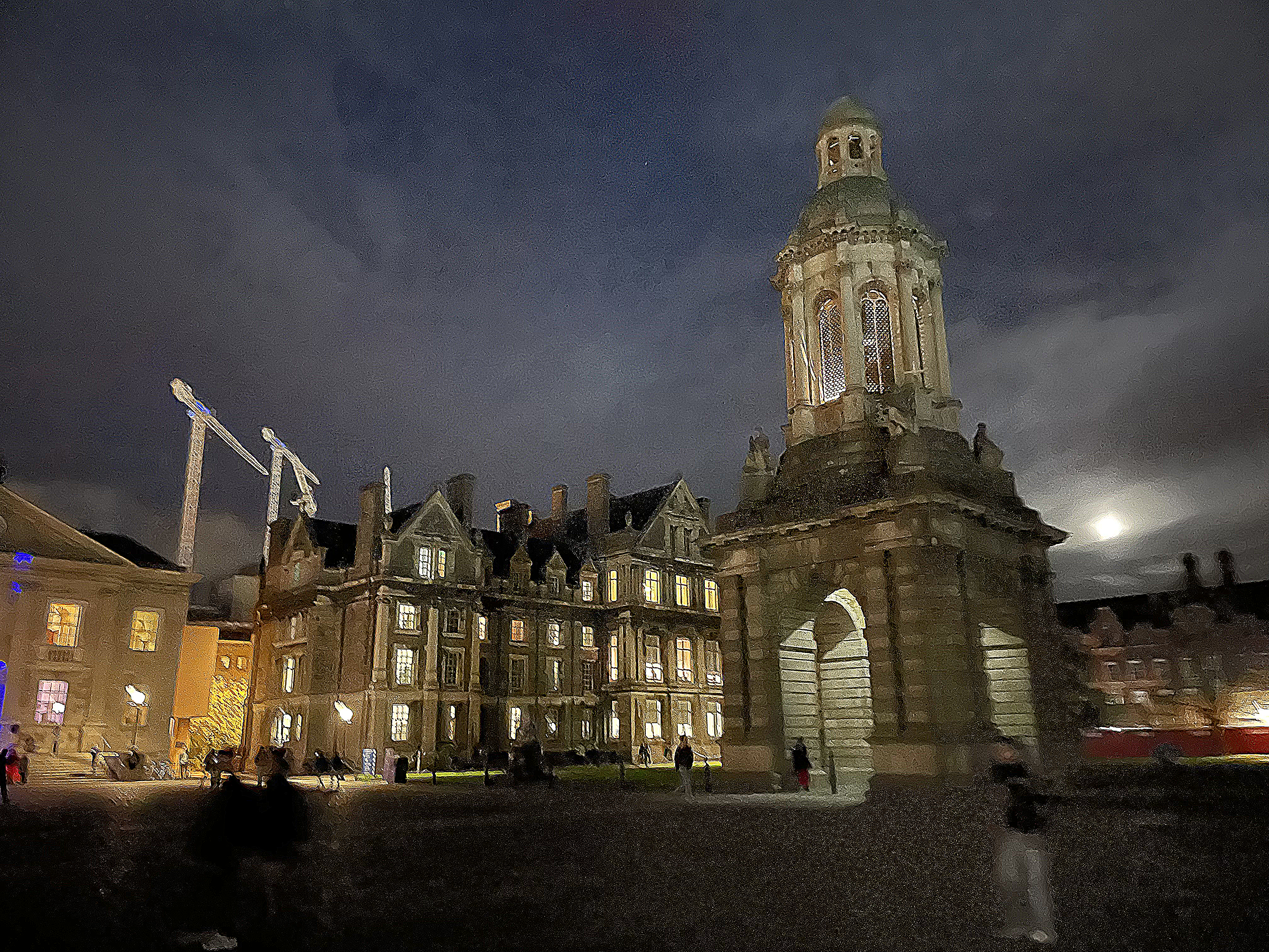
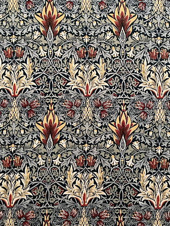
This project implements various filters, effects, and image processing methods in Python using the NumPy module. The project code has been written to reflect the logic behind the methods, not to maximise their internal efficiency.
Python is an interpreted language that takes enormous amounts of time to execute large nested loops. Therefore, NumPy has been used to speed up calculations. It does this by running the same operation in all the cells of an array in parallel.
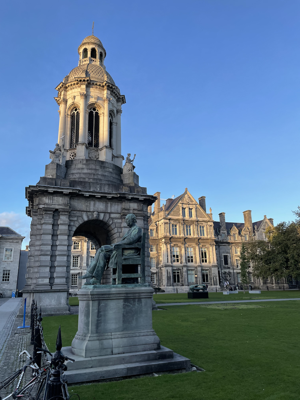
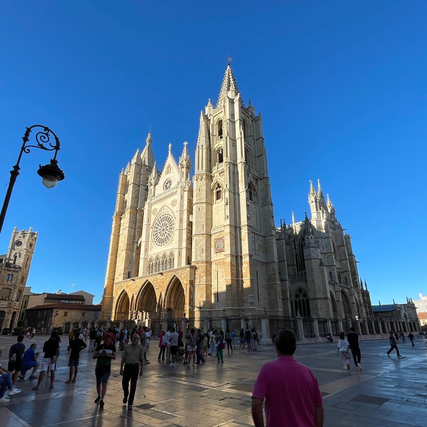
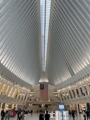
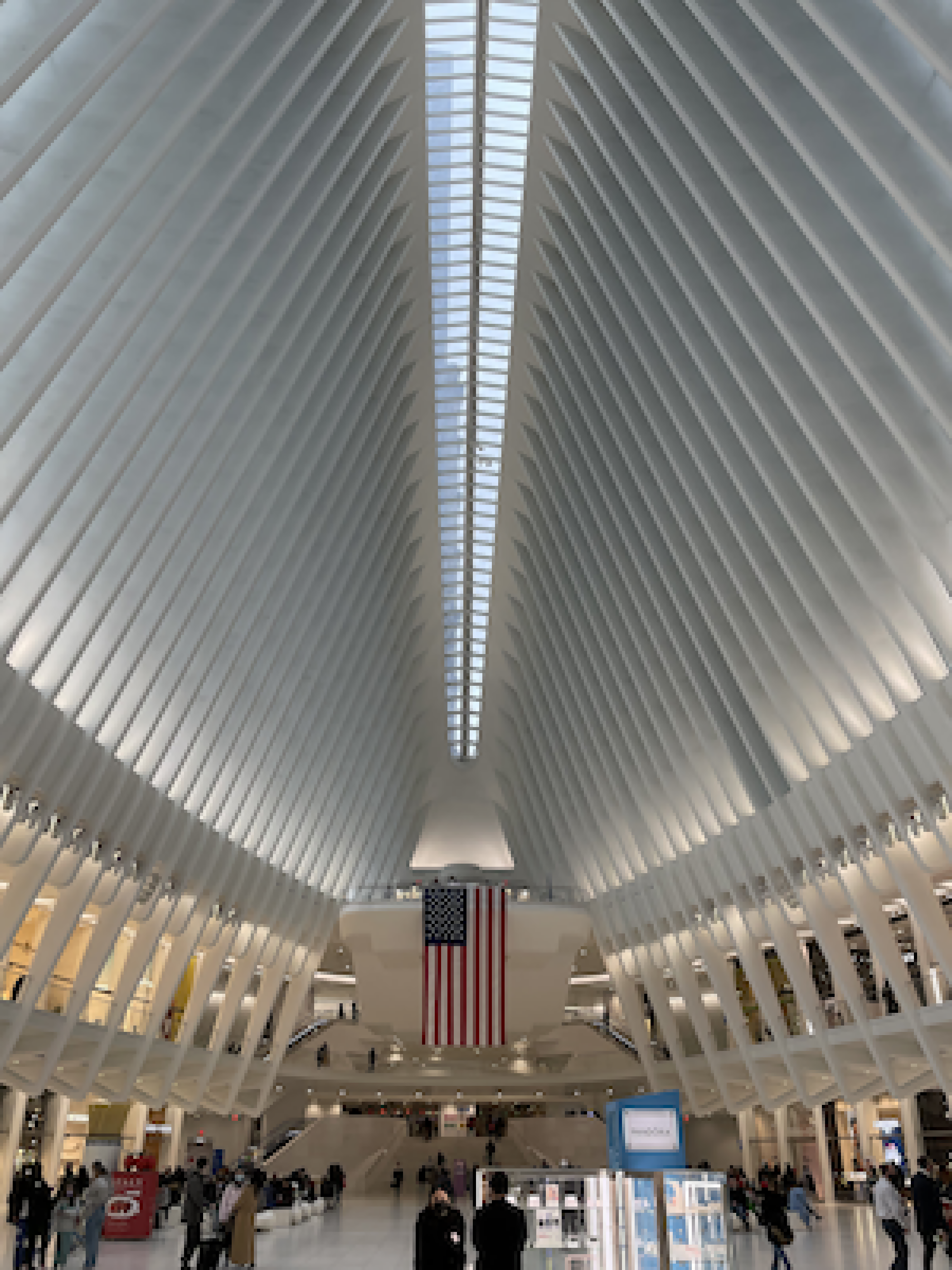
The images included in this report have been obtained from the author's camera roll. Many have been taken with different devices through the years, which explains the differences in quality between some images.
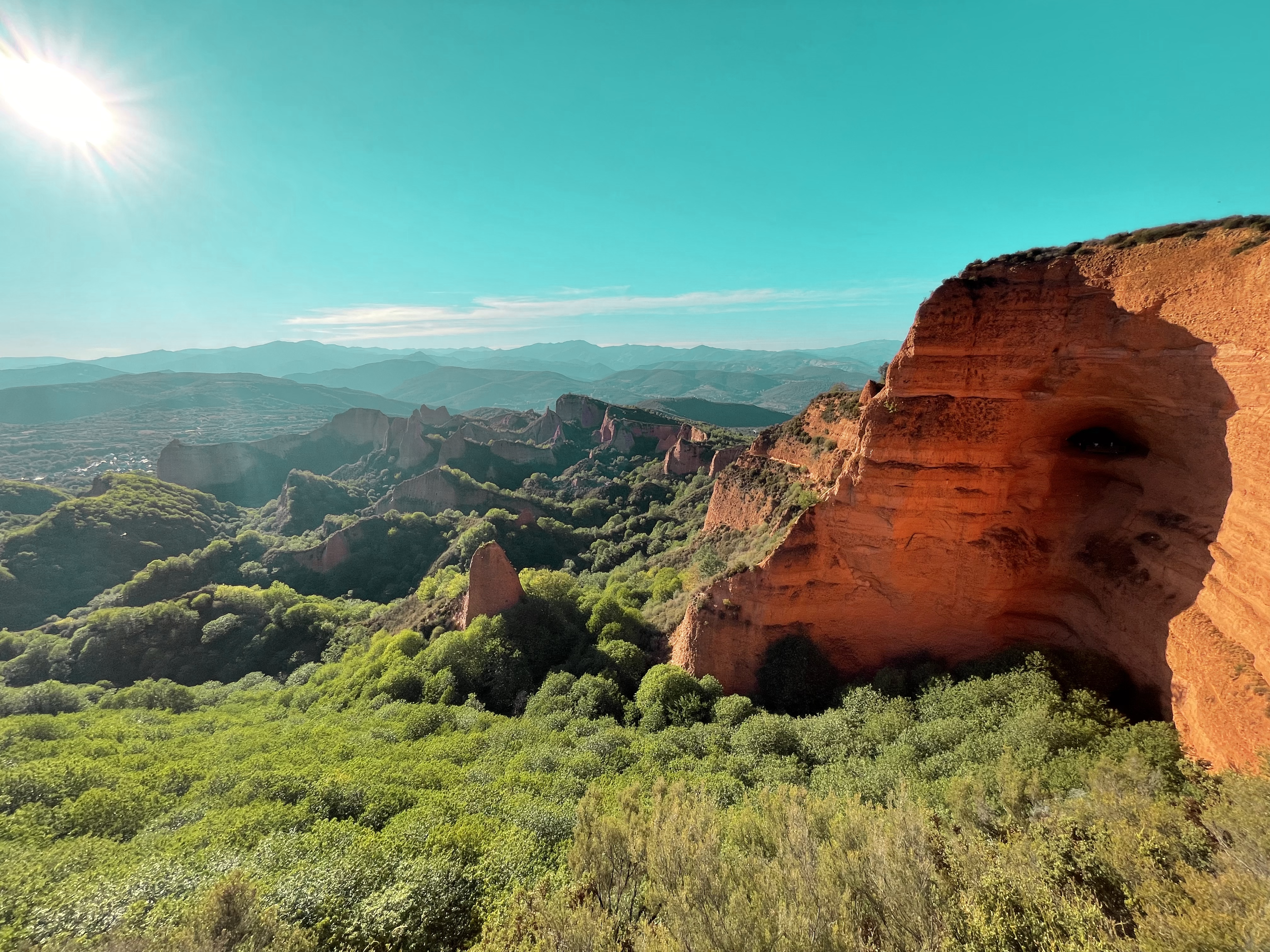
The images have been selected because they contain interesting elements for the experiments ---colours, shapes, noise, or others. The images that provided the most interesting results for the given method were used in each section.
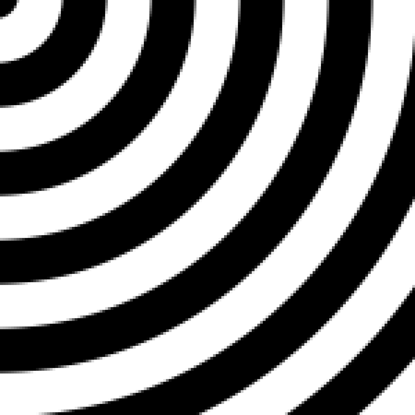
The synthetic images used to test rescaling methods were obtained from the TEST IMAGES dataset.
Saturation enhancement is an image processing technique for both technical and artistic purposes. For practical purposes, it can be used to correct colour blandness due to physical or optical causes. It can also help people with moderate colour blindness or visual impairments to visualise colours more easily. For artistic purposes, it is often used to give a sense of exuberance or to make photographs more attractive.
One of the most intuitive ways to implement this filter is to convert
the colour model from RGB to HSV or HSL. Therefore, conversions between
RGB, BGR, Grayscale, HSV, and HSL colour modes have been implemented for
this project. Actually, only the RGB
def split_channels(img):

    '''
    Split the channels of an image into separate images.

    Args:
        img (np.array): The image.

    Return:
        The channels in a tuple.
    '''

    number_of_channels = img.shape[2]

    return tuple([img[:, :, c] for c in range(number_of_channels)])

def merge_channels(channels):

    '''
    Merge the channels of an image into one single image.

    Args:
        channels (tuple): A tuple containing the channels to be merged.

    Result:
        The resulting image combined.
    '''

    return np.dstack((channels))

def saturation_apply_scale(img, scale):

    '''
    Scale the saturation channel of an HSL image img by the scale float.

    Args:
        img (np.array): An HSL image.
        scale (float):  An scaling float.

    Return:
        The image after modifying its saturation channel.
    '''

    # Convert the image to HSV.
    img_hsv = color_rgb_to_hsv(img)

    # Split the channels.
    h, s, v = split_channels(img_hsv)

    # Multiply the Saturation channel by the scale we decided.
    # We need to clip values that are out of range.
    s =  np.minimum(s * scale, np.ones_like(s))

    # Join the channels again.
    img_hsv = merge_channels((h, s, v))

    # Convert it back to RGB and return it.
    return color_hsv_to_rgb(img_hsv)
The code included above these lines shows the implementation of the saturation enhancement filter. It has been written following the functional style: to perform actions, it calls other functions. For example, the split_channels and merge_channels functions are almost NumPy aliases to operate with arrays more intuitively. These functions split or merge the colour channels of an image. Thus, an RGB image can be an MxNx3 matrix or three MxN matrices.
Thus, this code converts the image from RGB to HSV and separates the channels into three matrices H, S, and V. The S matrix is then used to operate. Next, each element in the S matrix is scaled using the scale parameter, whose result is clipped to 1 to avoid unwanted overflows in the final image. Finally, the resulting HSV image is converted to RGB again and returned.
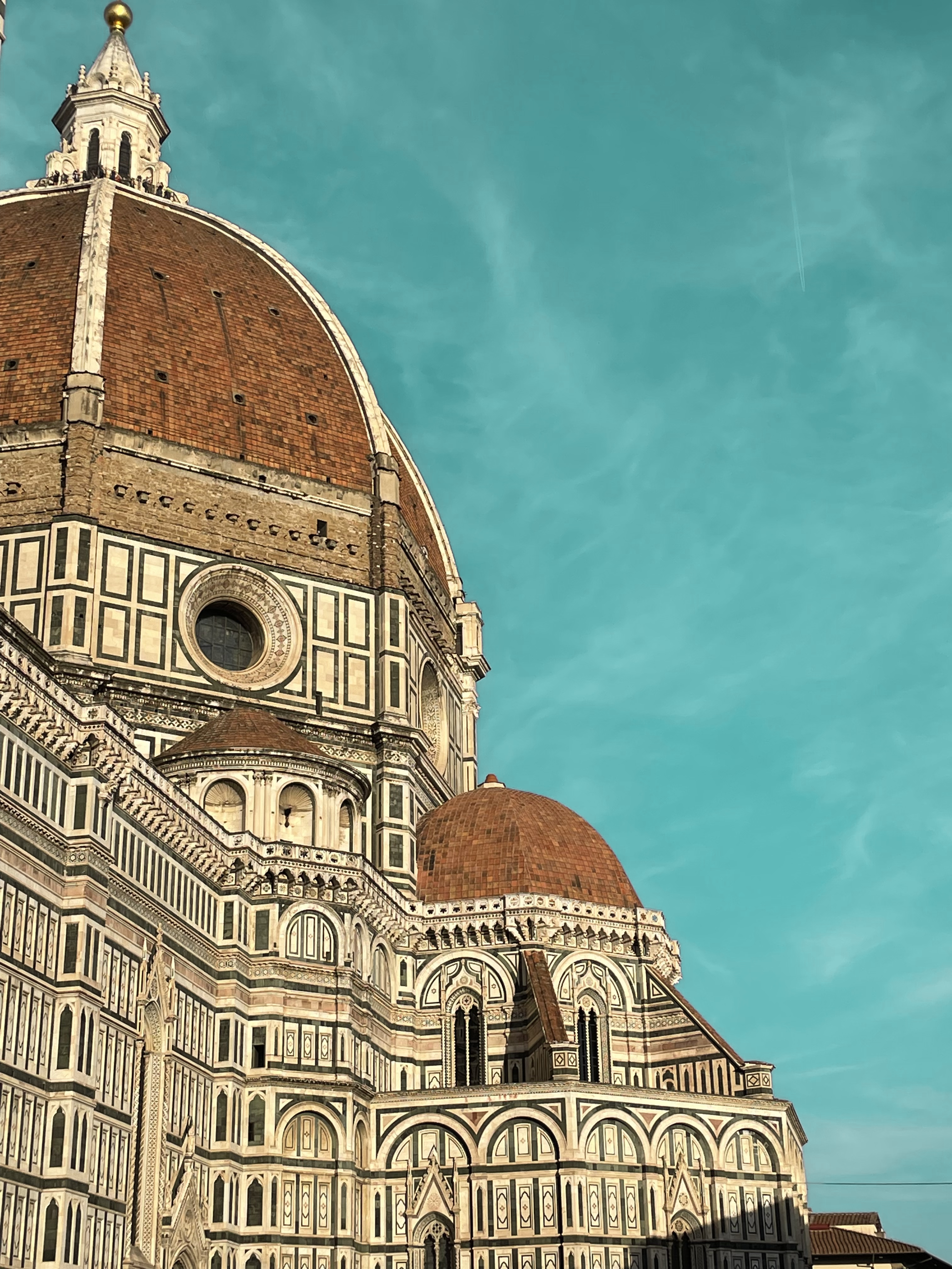
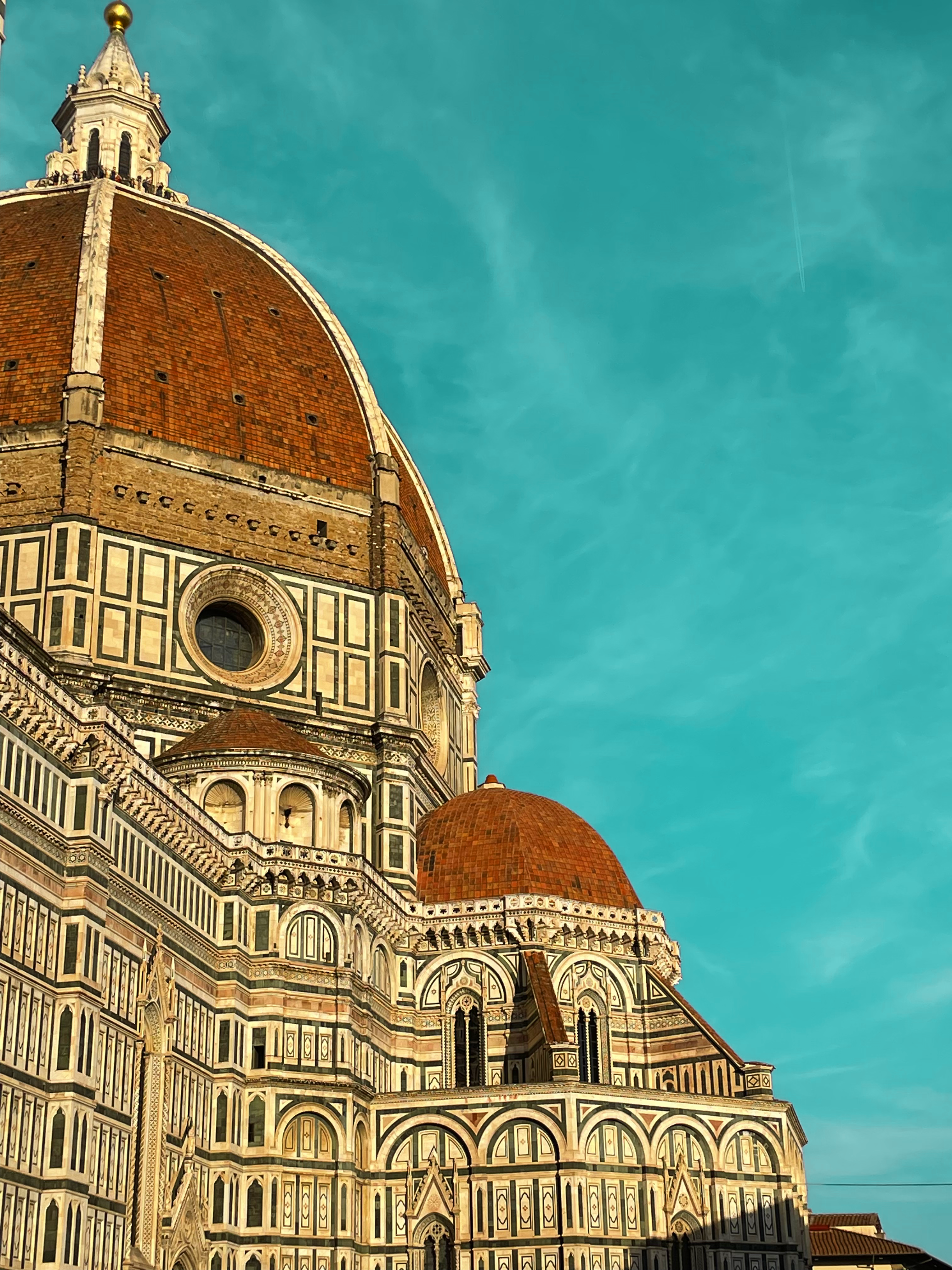
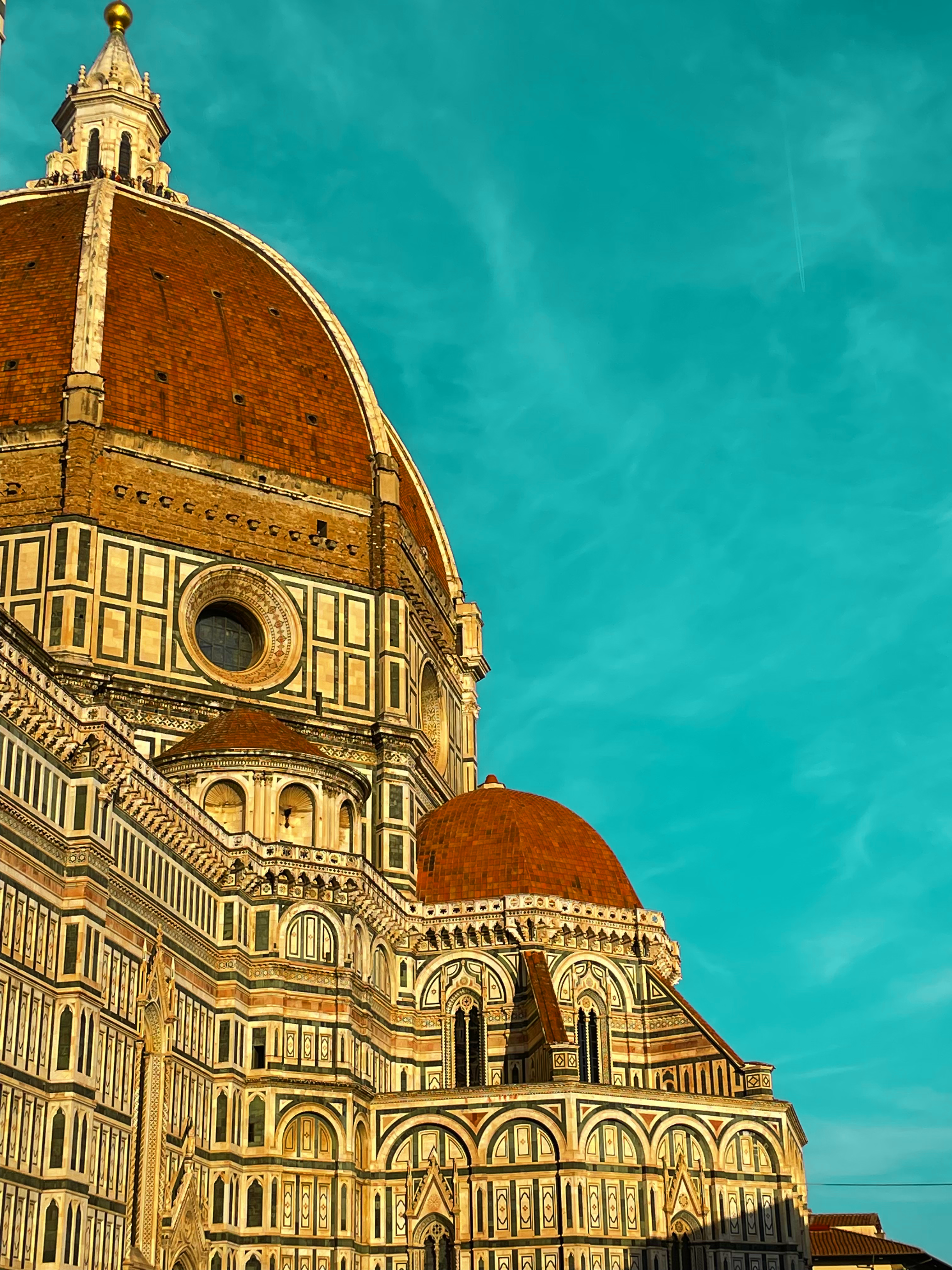
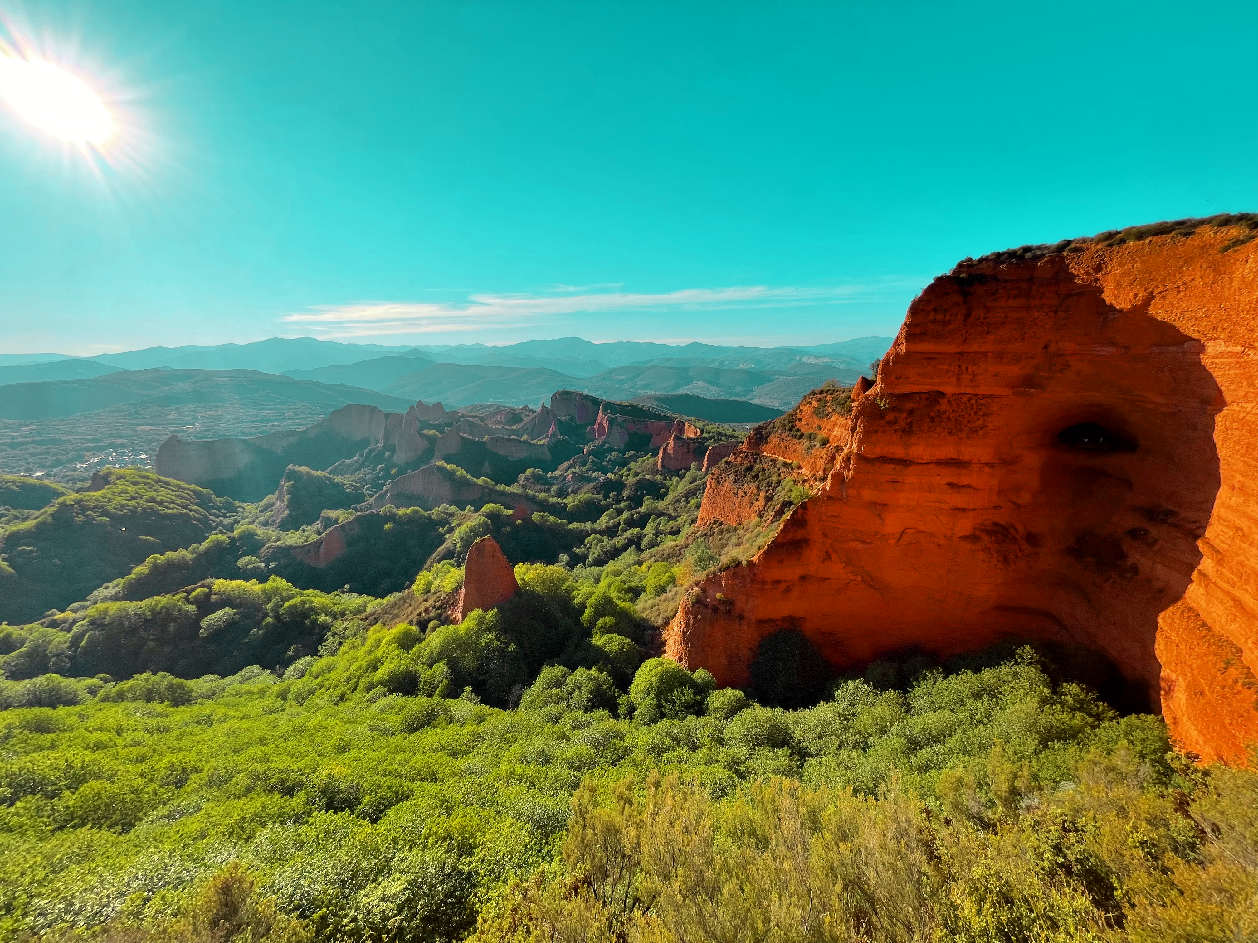
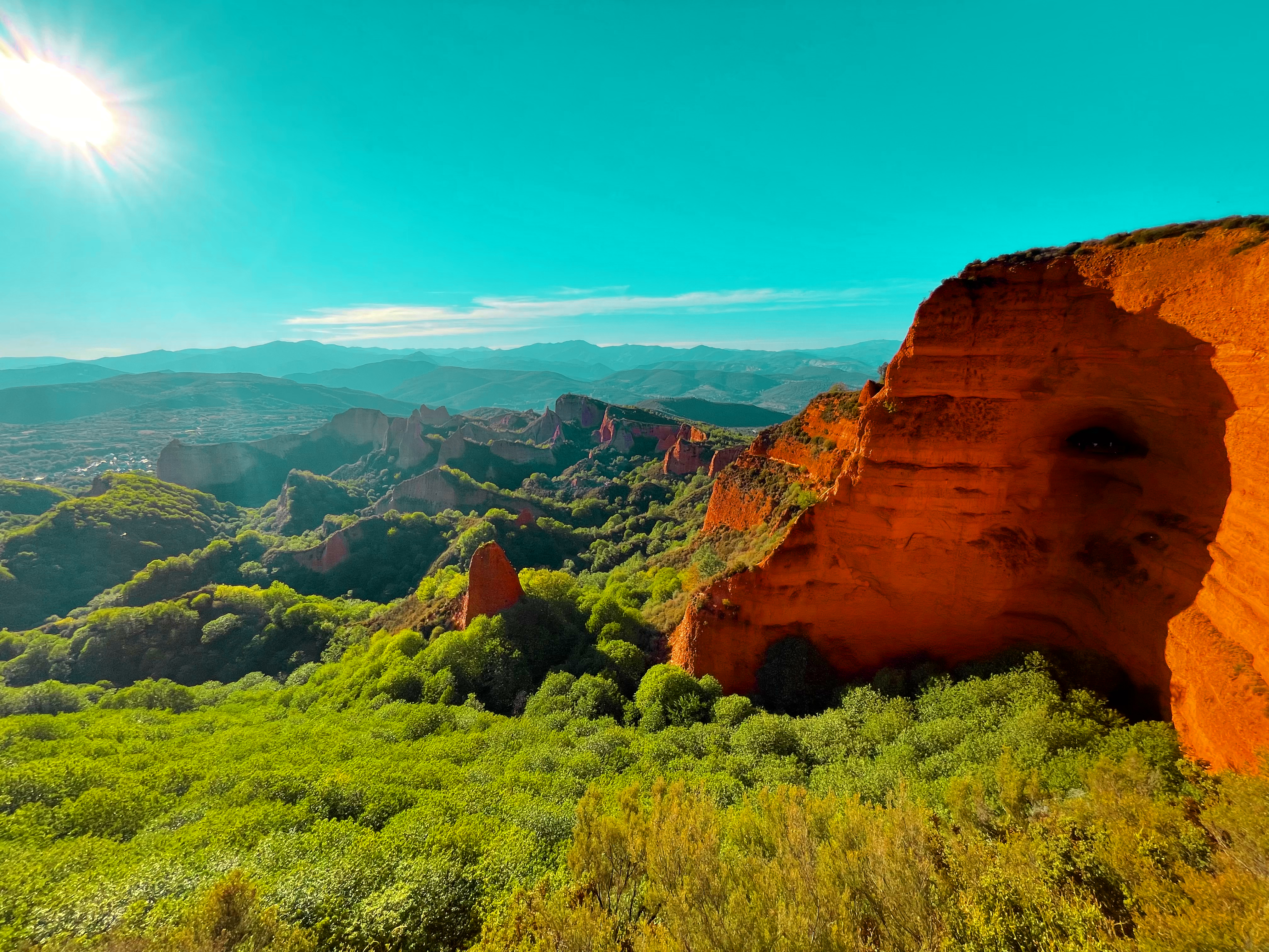
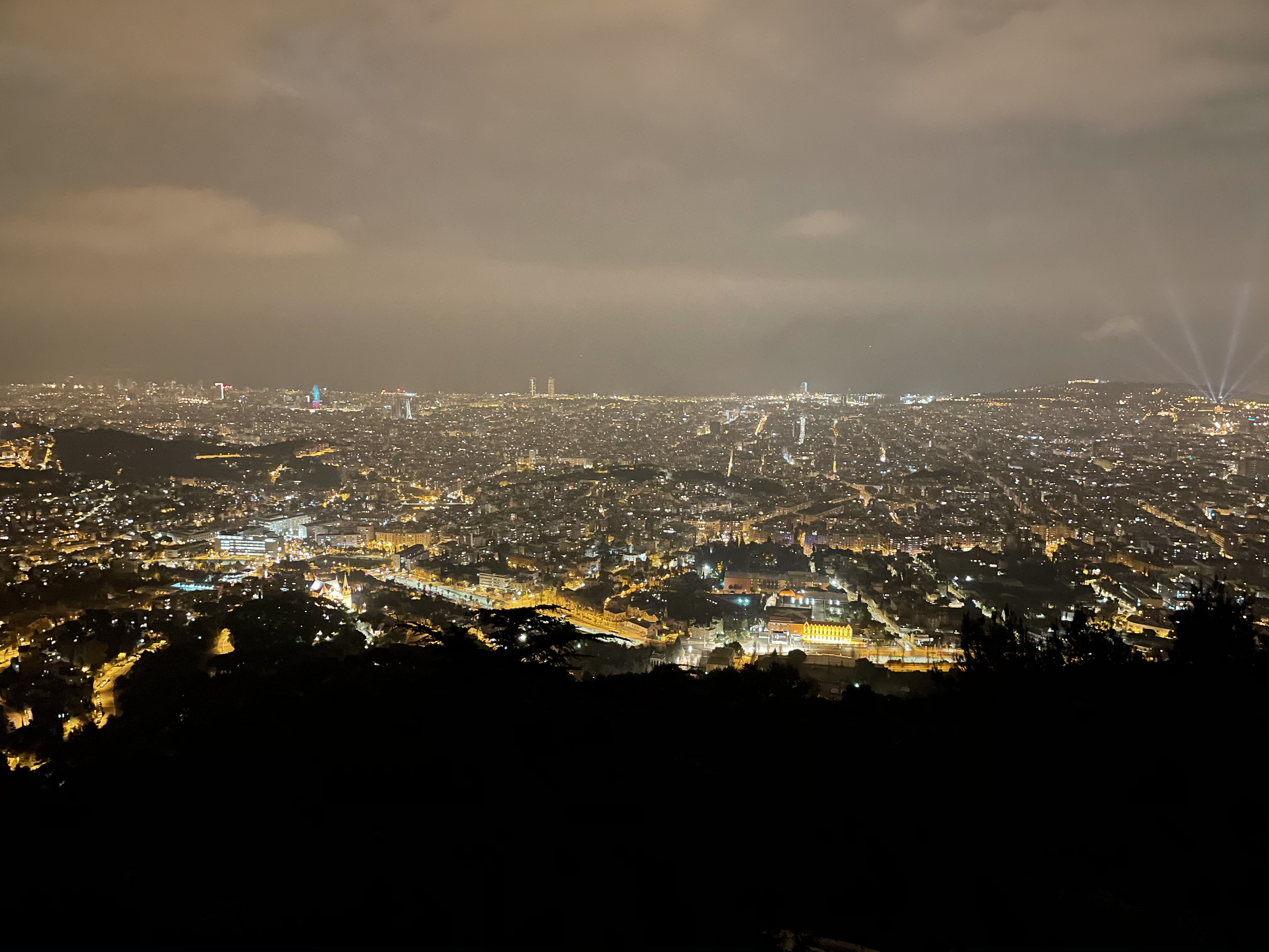
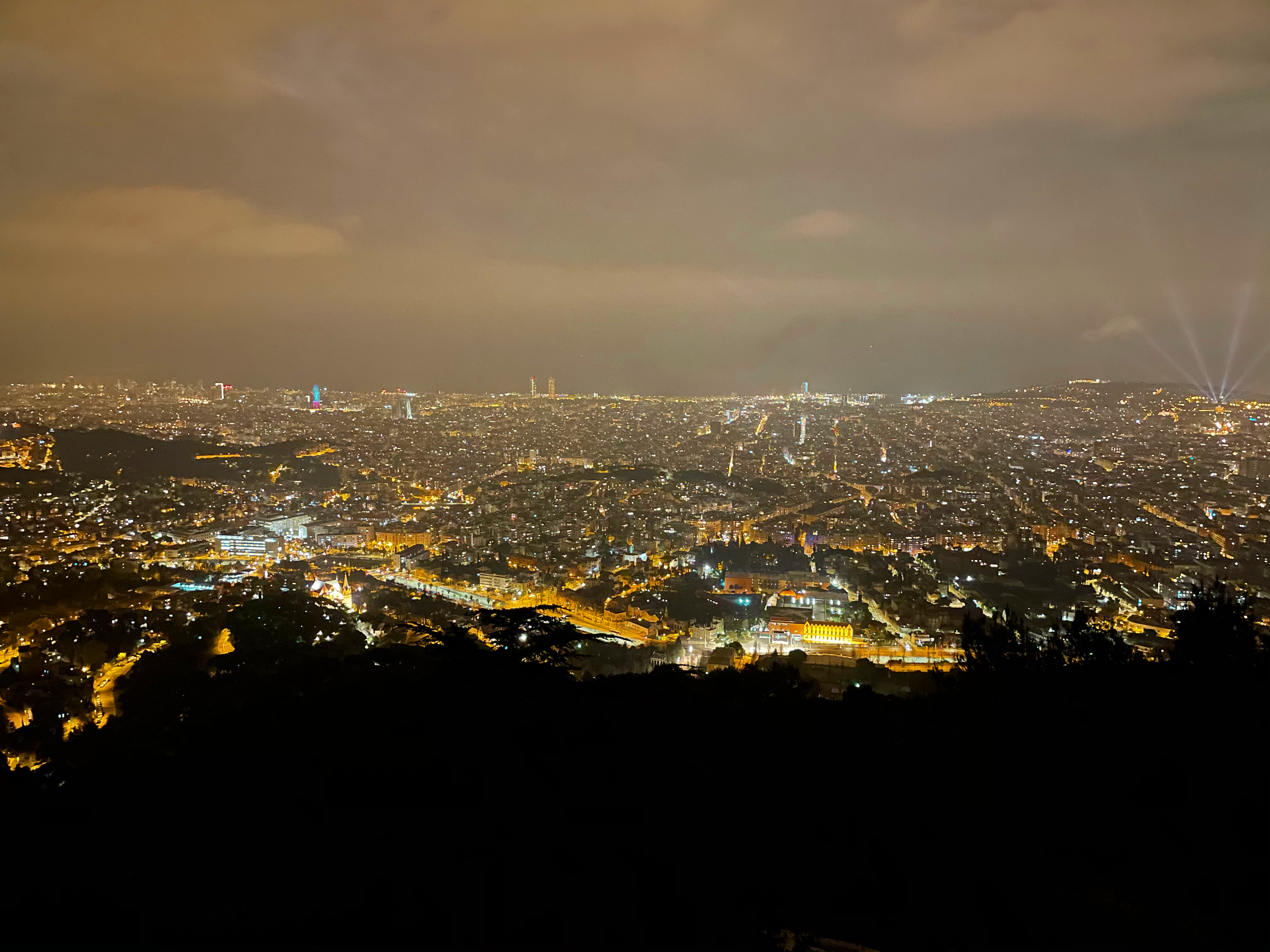
Saturation enhancement: (a) original image; (b) scale = 1.0; (c) scale = 1.5; (d) scale = 2.0. Saturation enhancement: (a) original image; (b) scale = 1.0; (c) scale = 1.5; (d) scale = 2.0. Saturation enhancement: (a) original image; (b) scale = 1.0; (c) scale = 1.5; (d) scale = 2.0.Figures 1{reference-type="ref" reference="fig:saturation_florence"}, 2{reference-type="ref" reference="fig:saturation_medulas"} and 3{reference-type="ref" reference="fig:saturation_skyline"} show the results of this filter on three different images using different scale parameters. A very noticeable difference in the blue tones of the images can be observed between the original image and the one filtered with scale=1.0. Intuitively, this should not occur. After reviewing the implementation and various articles, the conclusions are that this is due to a mismatch between the two colour models, as expressed by the formulas shown in Wikipedia (Wikipedia). The other shades, however, do show a direct correspondence.
It is interesting to note how the colours become much more vibrant as the scale parameter increases in the bottom two images of each Figure. As a counterpart, it can also be seen how the image noise becomes more visible in Figure 3{reference-type="ref" reference="fig:saturation_skyline"} as this parameter increases.
Duotone is a remarkably artistic filter. In the pre-digital era, there were already techniques to create this filter by post-processing. Nowadays, it is usually done using image editing programs such as Adobe Photoshop (here). It is widely used in commercial graphic design and editing for its visually attractive results.
This effect is based on converting a grayscale image to an image in a scale of two different colours. In other words, it is an image in which every pixel's brightness is used to interpolate two colours. In a conventional grayscale image, colours could be explained as a gradient between black and white. Duotone allows using any colour of the RGB spectrum for this purpose.
def duotone(img, color1, color2):

    '''
    Apply a duotone effect to the image.

    Args:
        img (np.array): A grayscale image.
        color1 (np.array):  'Shadows' RGB color.
        color2 (np.array):  'Lights' RGB color.

    Return:
        The image after applying the duotone.

    See:
        https://helpx.adobe.com/ie/photoshop/how-to/add-duotone-color-effect.html
    '''

    # Convert the image to gray.
    img = color_rgb_to_gray(img)

    # Normalize the image.
    img_norm = img / 255

    # Push the extrems to 0 and 1.
    img_norm = img_norm - np.min(img_norm)
    img_norm = img_norm / np.max(img_norm)

    # The basic formula for interpolation is n1 + (n2 - n1) * step.
    # We will do this with NumPy.

    # Create two images of pure color1 and pure color2.
    img_color1 = np.ones((img.shape[0], img.shape[1], color1.shape[0]), int)
    img_color1 *= np.array(color1, dtype='uint8')

    img_color2 = np.ones((img.shape[0], img.shape[1], color2.shape[0]), int)
    img_color2 *= np.array(color2, dtype='uint8')

    # Apply the interpolation function.
    step = merge_channels((img_norm, img_norm, img_norm))
    return np.array(color1 + (color2 - color1) * step, dtype='uint8')
The code above these lines shows the implementation of the duotone filter. First, the image is converted to grayscale to get the brightness of each pixel in a matrix. This array is then normalised so that the values are decimals from 0 to 1. For more striking results, the minimum value is pushed to 0 and the maximum to 1. Finally, two arrays containing the pure colours are created, and the brightness matrix is used as the step in the colour interpolation.
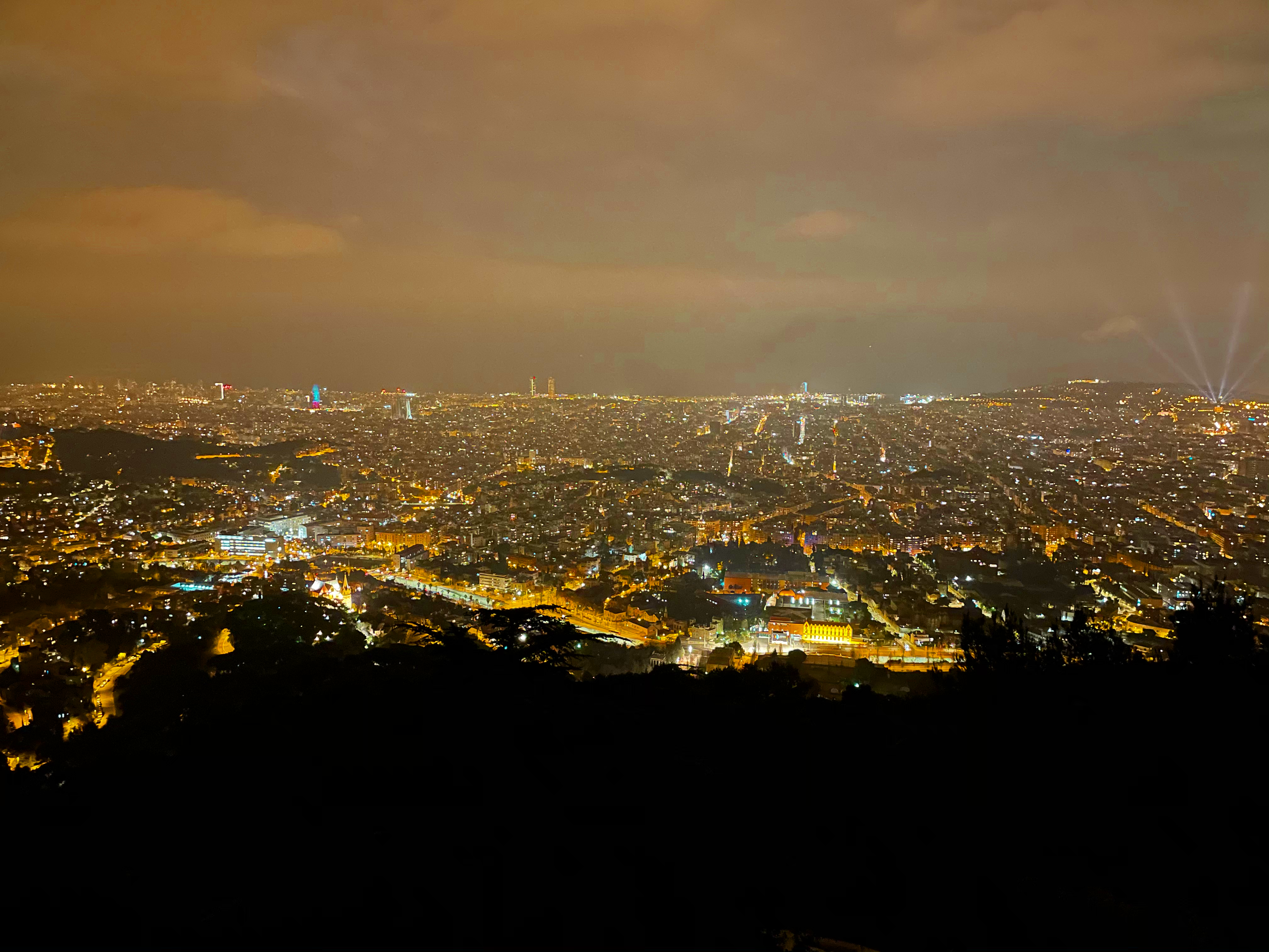
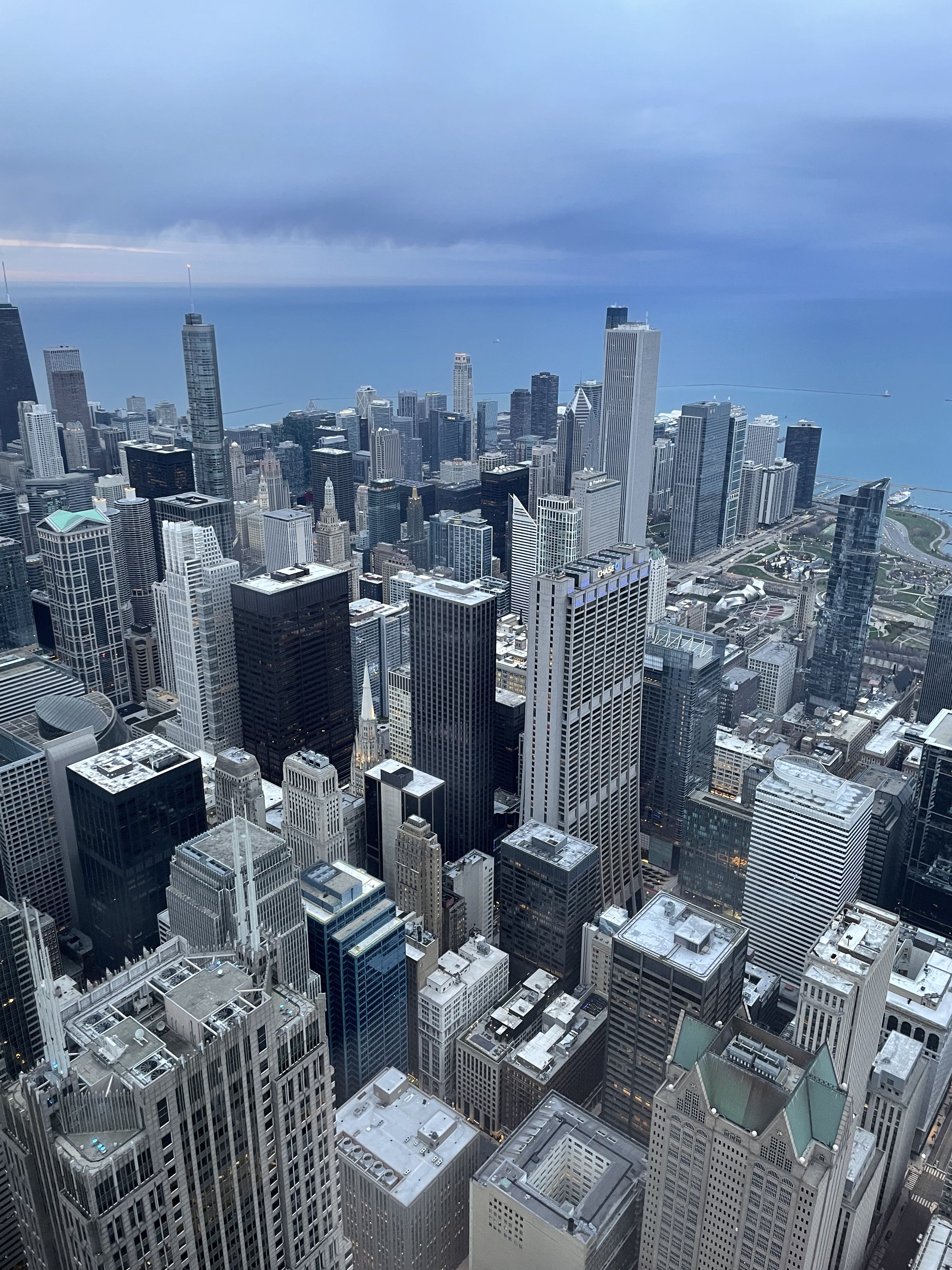
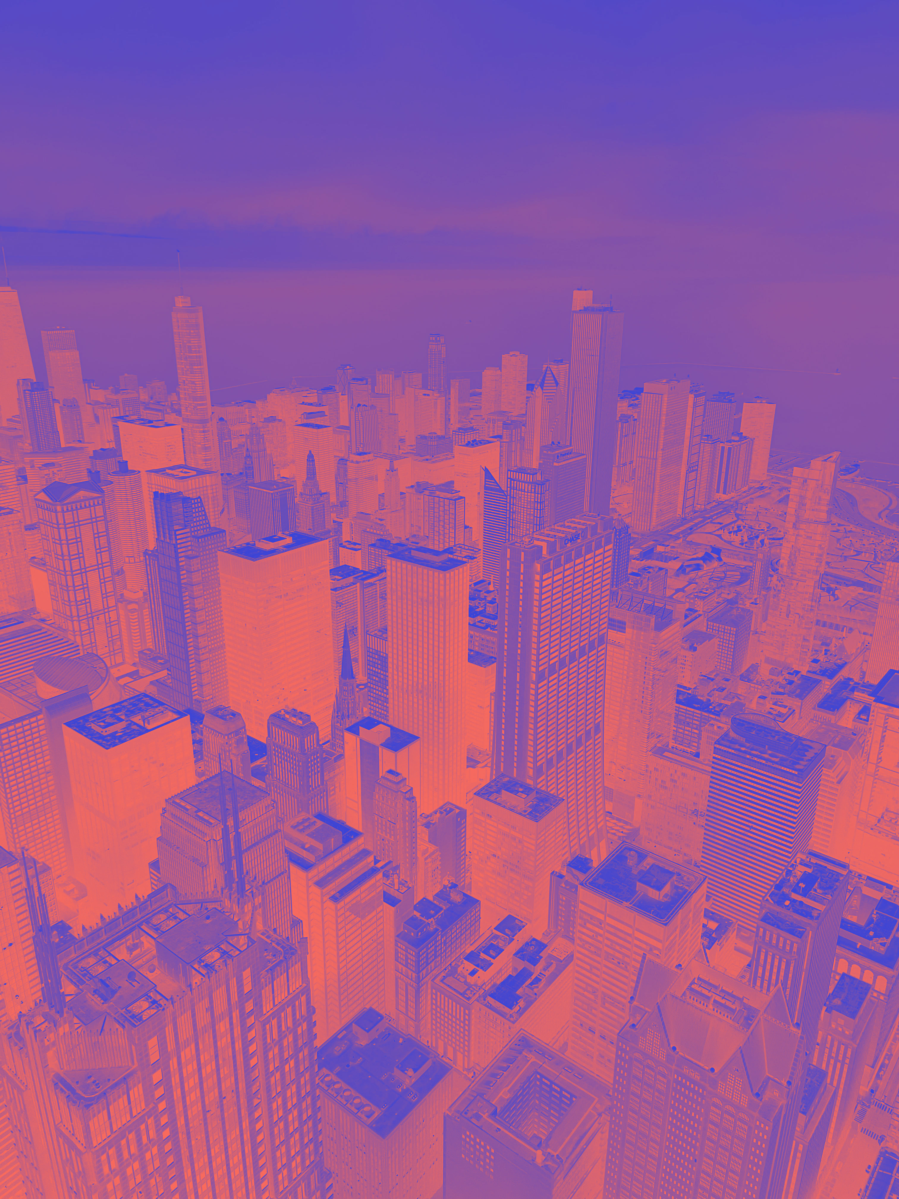
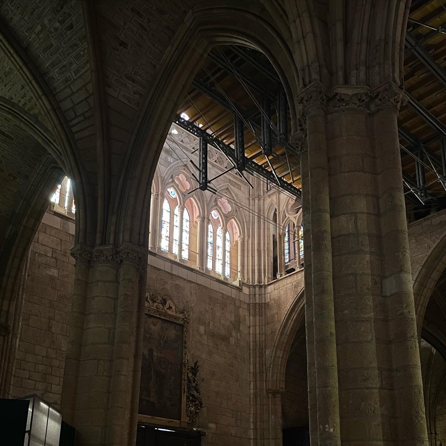
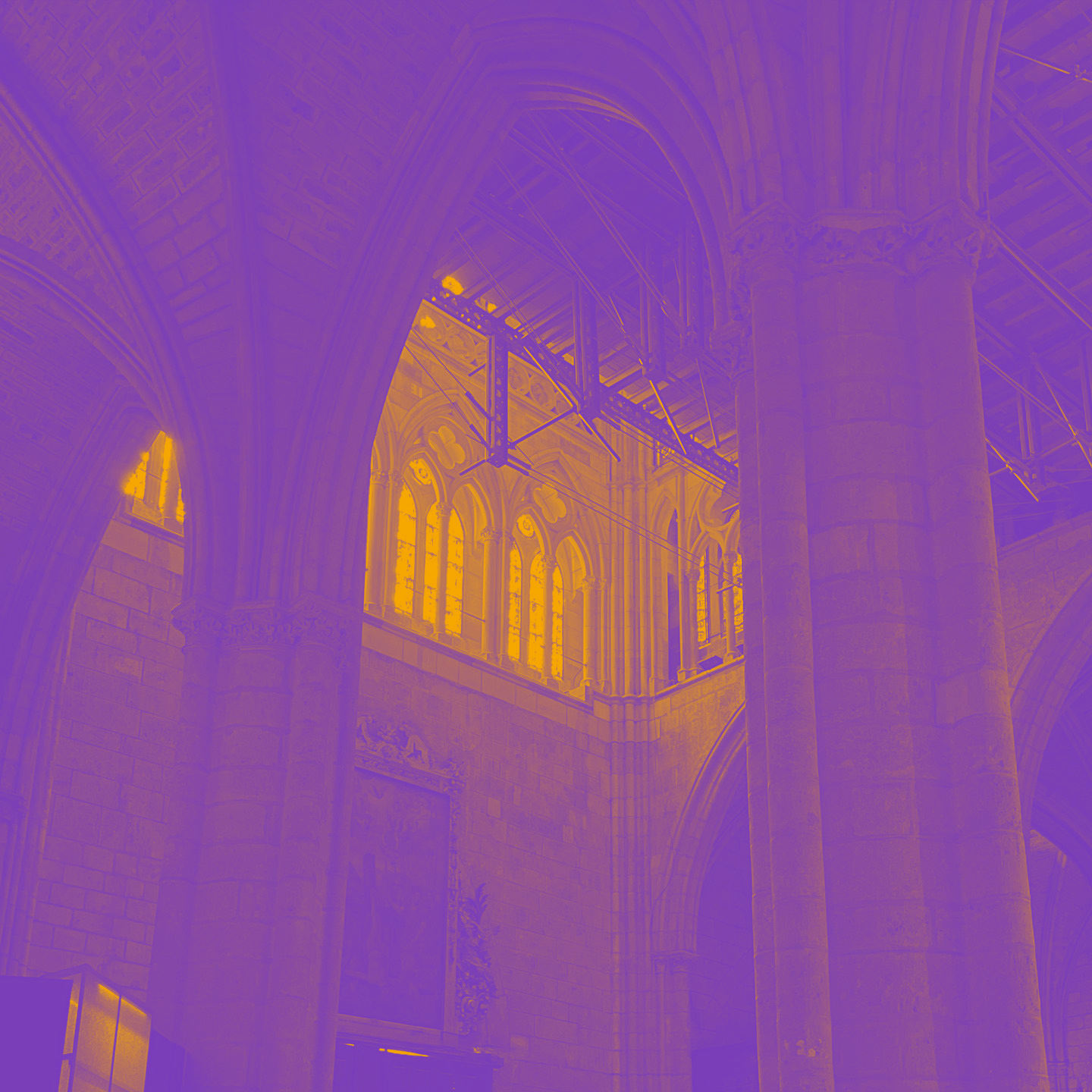
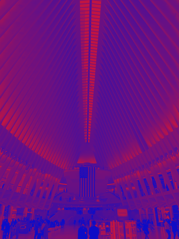
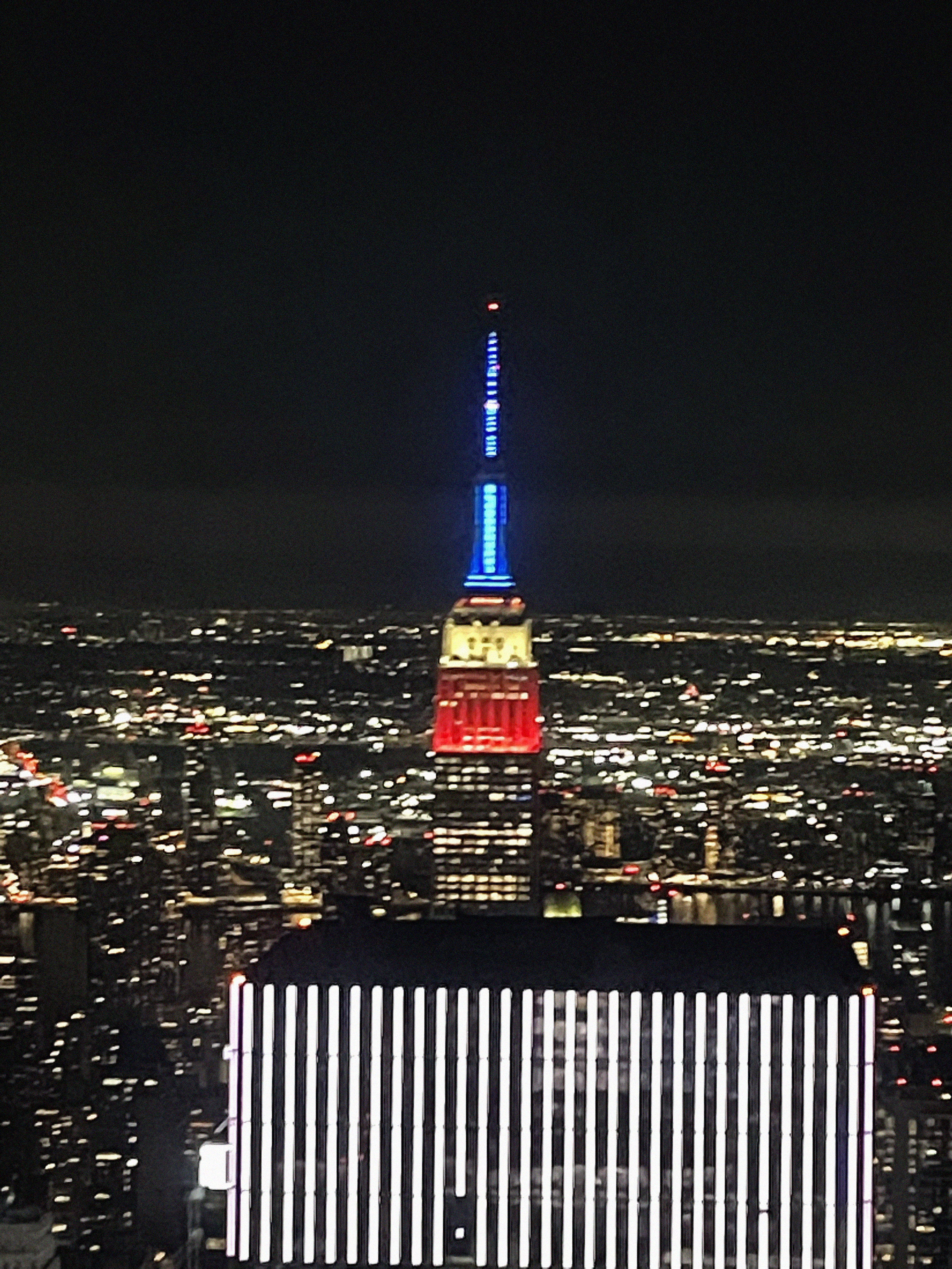
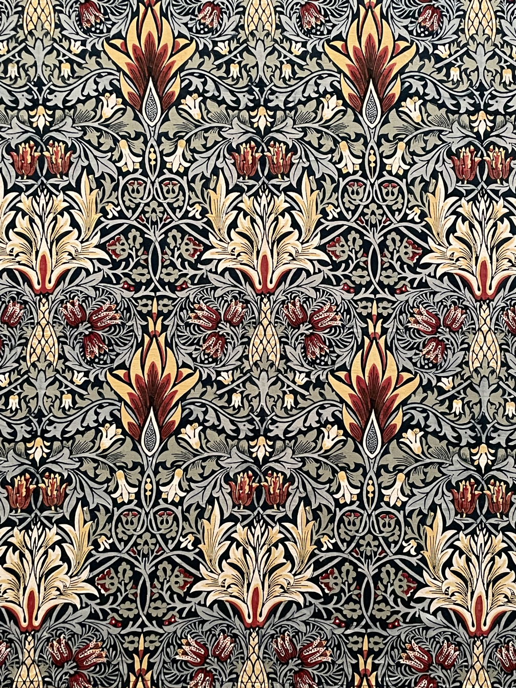
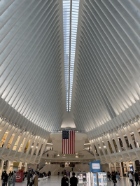
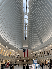
Duotone effect: (a) original image; (b) red and purple duotone. Duotone effect: (a) original image; (b) yellow and purple duotone. Duotone effect: (a) original image; (b) blue and red duotone.Figures 4{reference-type="ref" reference="fig:duotone_chicago"}, 5{reference-type="ref" reference="fig:duotone_leon"} and 6{reference-type="ref" reference="fig:duotone_nyc"} show the results of this filter on three different images using different interpolating colours. These filters obtain a striking version of the image when used with cautiously selected colours, as they get unexpected contrasts from the original image.
The stained glass filter is an essentially artistic effect. It obtains a visually intriguing result where pixels are grouped together with other nearby pixels to form homogeneous colour groups using the average of their original colours. The result is an image similar to a stained glass pattern or the result of viewing the image through translucent and irregular glass.
This effect is obtained by creating a series of generator points and grouping the pixels of the image according to their closest generator point.
def stained_glass(img, pnts):

    '''
    Apply a stained glass effect.

    Args:
        img (np.array): An RGB image.
        pnts (int): The number of generating points in the stained glass effect.

    Return:
        An image after applying the stained glass effect.
    '''

    # Get the dimensions. We do not mind the depth. It will be handled by func.
    height = img.shape[0]
    width = img.shape[1]

    # Get the position of the generating points.
    gen_points = np.array([(randint(0, height), randint(0, width)) for x in range(pnts)])

    # Get all X and Y pixel indices in an array.
    # This means that pixel_indices[Y, X] = [Y, X].
    pixel_indices = np.indices((height, width))
    pixel_indices = merge_channels((pixel_indices[0], pixel_indices[1]))

    # Init the datastructure to store the closest point yet and the minimum distance.
    closest_labels = np.zeros((height, width))
    minimum_distances = np.matrix(np.ones((height, width)) * np.inf)

    # Iterate by all the generating points.
    for i, gen in enumerate(gen_points):

        # Now get the euclidian distance from each pixel in the image to the gen point.
        # We can do this using NumPy.
        gen_distances = np.sum((pixel_indices - gen) ** 2, axis=2)

        # Everywhere where this distance is shorter than the current minimum distance, get indices.
        change_labels = gen_distances < minimum_distances

        # Use those indexes to store the new minimum distances and minimum labels.
        closest_labels[change_labels] = i
        minimum_distances[change_labels] = gen_distances[change_labels]

    # Init the return variable.
    ret_img = np.zeros_like(img)

    # Iterate by all the generating points.
    # Now all the points in closest_labels have been correctly set.
    for i, gen in enumerate(gen_points):

        # Get all the colors summed and all the label counts to compute the average color of the
        # area.
        area_ind = closest_labels == i
        avg_colors = np.mean(img[area_ind], axis=(0))

        # Get the average color and put in on all those positions of ret_img corresponding to those
        # pixels.
        ret_img[area_ind] = avg_colors

    return ret_img
The code above these lines shows the implementation of the window filter. First, a series of generator points are generated in the range of the image. Then, using a loop, the geometric distance of each pixel to each generator point is obtained, and it is determined which point has the minimum distance to each pixel. Within this loop, each pixel is labelled with the index of the generating point assigned to it. Finally, for each generating point, the average colour of all its pixels is computed, and the newly calculated average replaces the original colour.
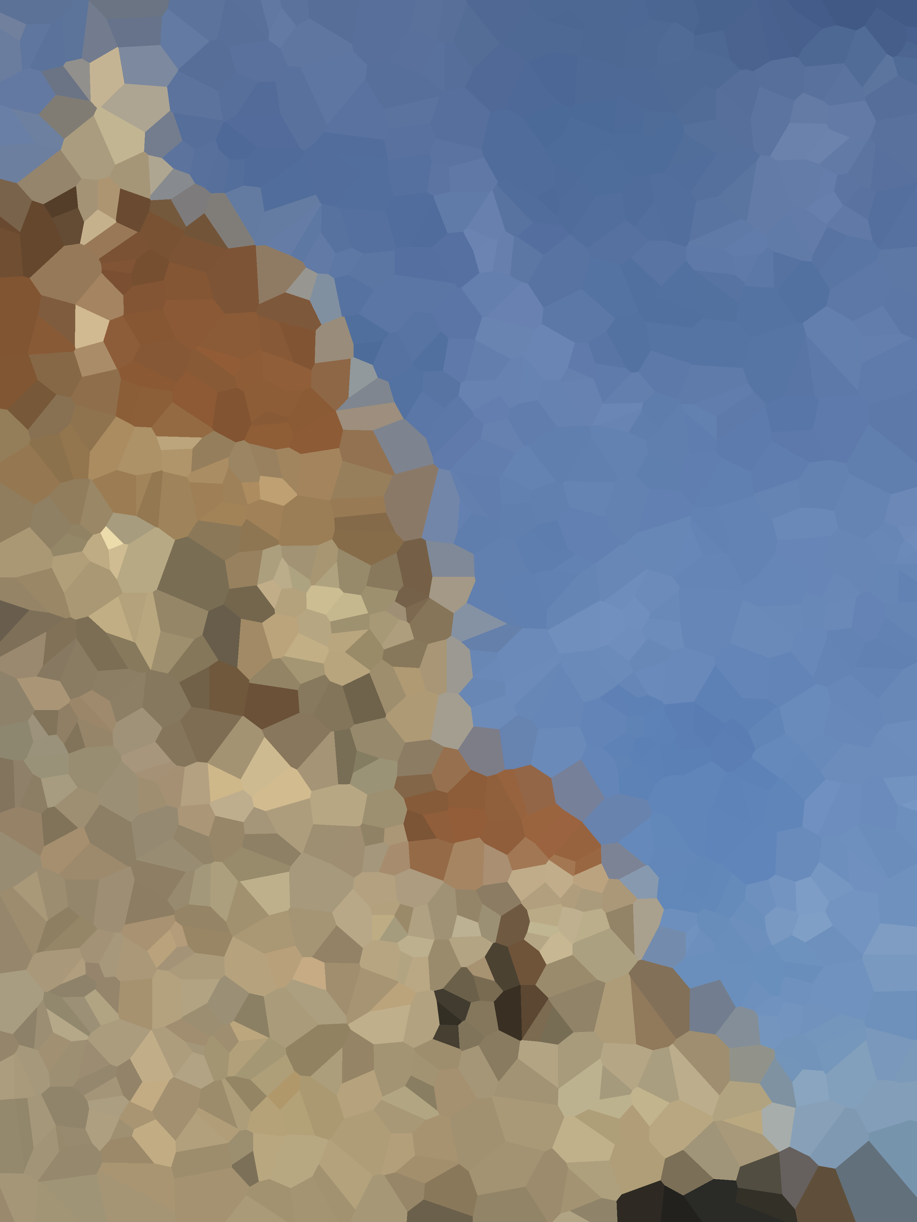
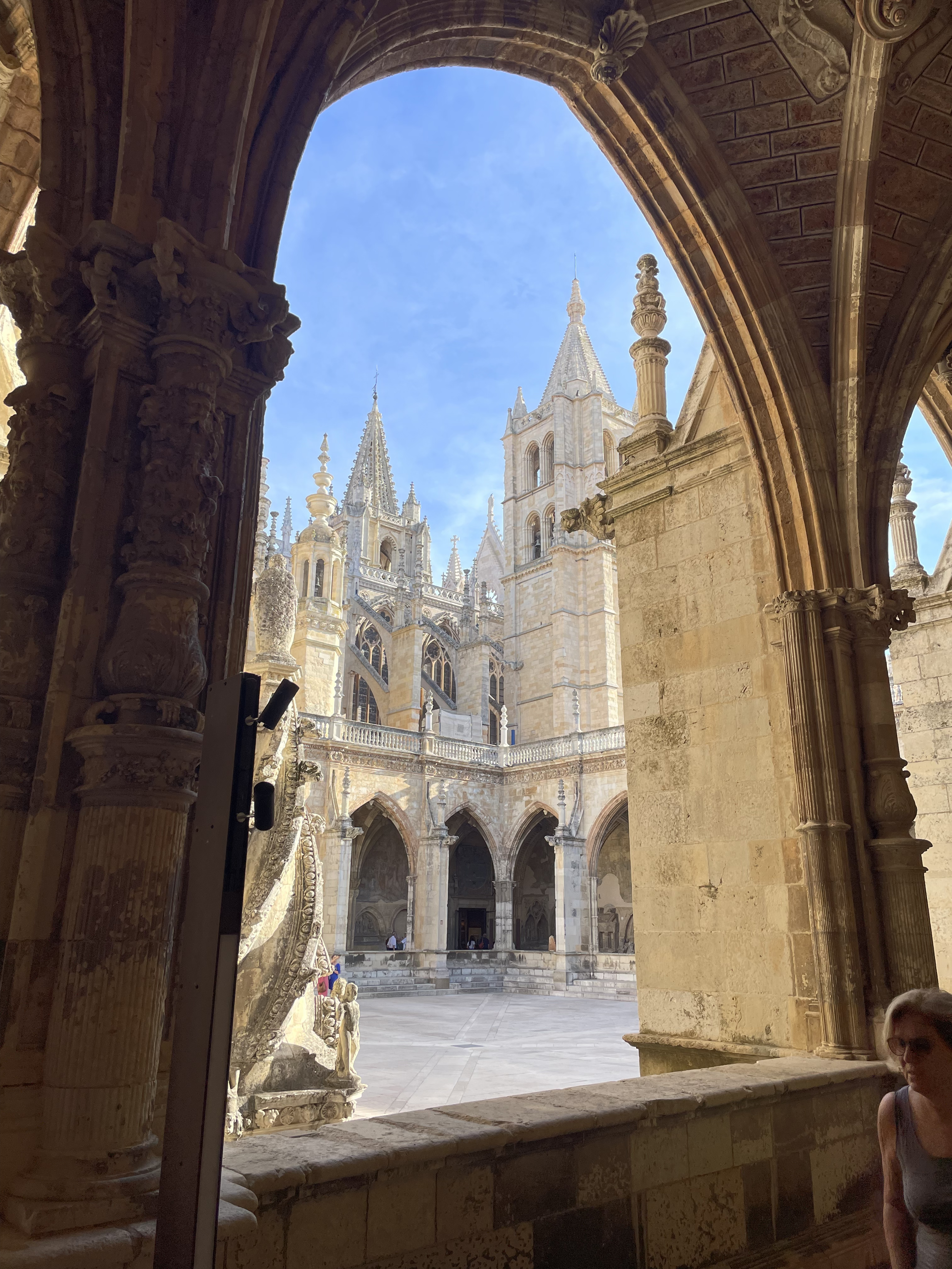
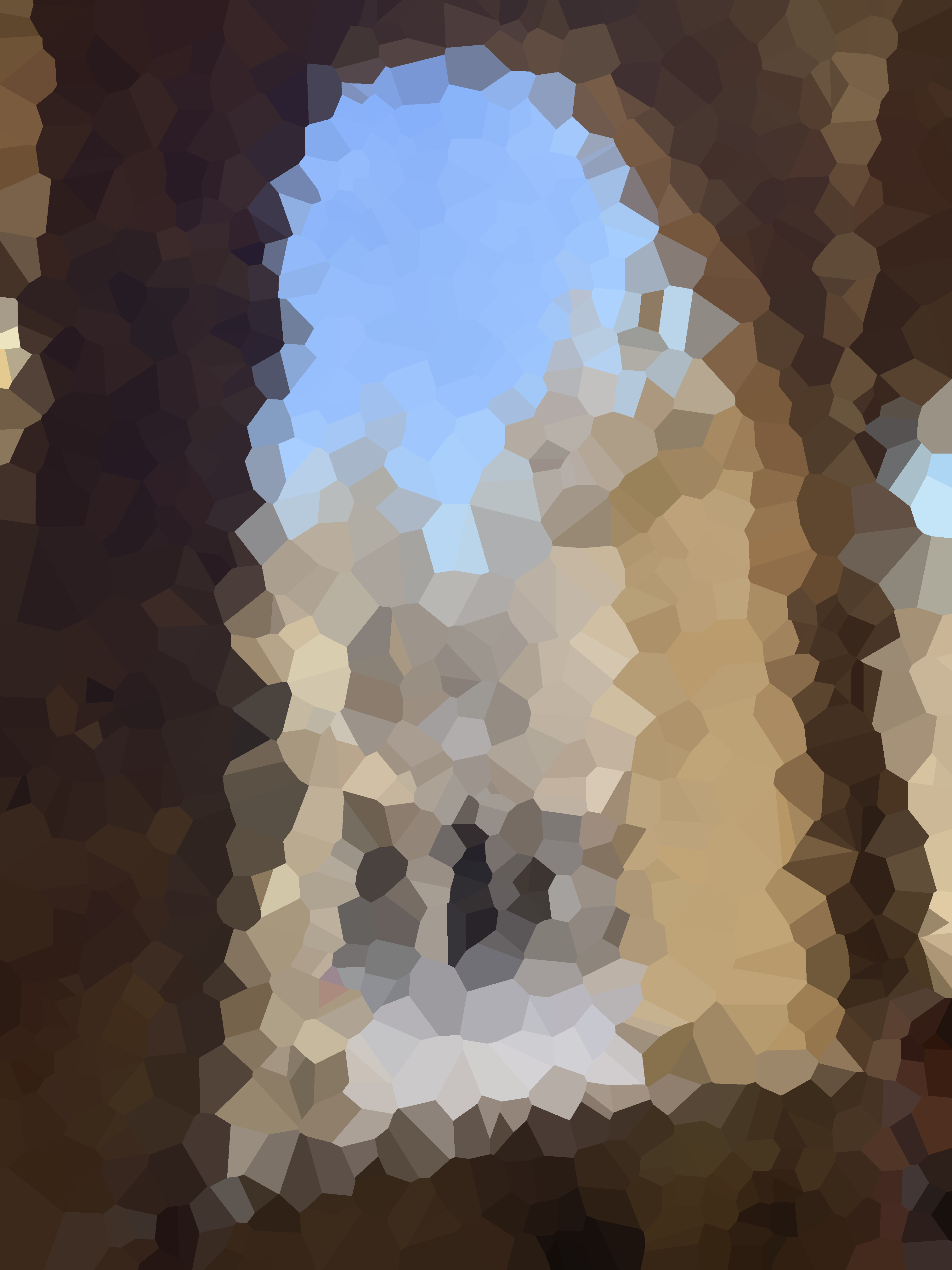
Stained glass effect: (a) original image; (b) stained glass effect. Stained glass effect: (a) original image; (b) stained glass effect. Stained glass effect: (a) original image; (b) stained glass effect.Figures 7{reference-type="ref" reference="fig:stained_glass_florence"}, 8{reference-type="ref" reference="fig:stained_glass_medulas"} and 9{reference-type="ref" reference="fig:stained_glass_leon"} show the results of this filter on three different images. These filters obtain an odd-looking version of the image that looks intriguing and not trivial. The shapes of the main objects can still be appreciated, although heavily distorted. The more minor details of the images are mostly lost due to the nature of the filter. An exciting aspect of this filter is its random nature, as every iteration will obtain a slightly different result.
The embossing effect results from convolving an image with one of the well-known embossing kernels. This effect highlights pixel-by-pixel colour differences to create an embossed or highlighted feel. This filter has artistic applications---it creates an interesting image when applied---and it also has practical uses. It can be used to enhance the contrasts in an image, to create bump maps from images, and for many other uses.
There are different emboss kernels by diameter and direction ---they can be vertical, horizontal, or mixed. In this project, mixed emboss kernels have been implemented where a vertical, a horizontal, and a vertical kernel are combined.
This filter is the first example of a convolution introduced in this project. Therefore, the methods to convolve an image are explained below this lines, although they are used all across the project.
def convolve(img, kernel, pad=True):

    '''
    Performs a kernel convolution on image img using the kernel.

    Args:
        img (np.array):  An image as a numpy array. It is one-dimensional or 3 dimensional.
        kernel (np.array): The kernel that will be used to compute the convolution.
        pad (Boolean): Whether to add padding before convolving or not.

    Return:
        The convolved image.
    '''

    # Get the kernel size.
    kernel_height = kernel.shape[0]
    kernel_width = kernel.shape[1]

    # Get the padding sizes.
    pad_y = kernel_height // 2
    pad_x = kernel_width // 2

    # Apply the padding to the image if it was set to true.
    if pad is True:
        img = np.pad(img, ((pad_y, pad_y), (pad_x, pad_x)), mode='edge')

    # Get the image size.
    img_height = img.shape[0]
    img_width = img.shape[1]

    # Get the convolved image sizes.
    conv_height = img_height - (kernel_height - 1)
    conv_width = img_width - (kernel_width - 1)

    convolved_image = np.zeros((conv_height, conv_width))

    for y in range(kernel_height):
        for x in range(kernel_width):

            # Get the end index.
            # This is the index next to the last one we want to get.
            end_y = img_height - (kernel_height - y) + 1
            end_x = img_width - (kernel_width - x) + 1

            # Get the current submatrix.
            submatrix = img[y:end_y, x:end_x]

            # Add the current submatrix, multiplied by the kernel element.
            convolved_image = convolved_image + (submatrix * kernel[y, x])

    return convolved_image

def convolve_all_channels(img, kernel, pad=True):

    '''
    Performs a kernel convolution on the N channels of image img using the kernel.

    Args:
        img (np.array):  An image as a numpy array. It is one-dimensional or 3 dimensional.
        kernel (np.array): The kernel that will be used to compute the convolution.
        pad (Boolean): Whether to add padding before convolving or not.

    Return:
        The convolved image.
    '''

    # Split the channels.
    channels = split_channels(img)

    # Apply the convolution to all channels.
    channels = [convolve(c, kernel, pad) for c in channels]

    # Join the channels again.
    return merge_channels(channels)
Above these lines are the convolve and convolve_all_channels functions. The convolve function is essential in this project, as it is used throughout all the remaining sections. This implementation seeks to speed up the execution of convolutions using NumPy while allowing the main logic of the convolution algorithm to be seen. The original convolution algorithm consists of 4 nested loops traversing the rows and columns of the original image and the rows and columns of the kernel. The main difference between the implementation shown here and the original algorithm is that the operations for all the image cells are executed in parallel. Instead of fetching one cell at a time and operating on a single kernel element, we fetch all cells simultaneously and operate on the kernel element. This computed cell array is added to the convolved_image accumulator.
The convolve_all_channels function is just a helper function that separates the three channels using the split_channels and merge_channels functions to perform a convolution on each channel using the kernel.
def emboss(img, kernel_size):

    '''
    Implements an emboss filter in n-dimensions.

    Args:
        img (np.array): An RGB image.
        kernel_size (number): Size of the kernel to be generated.

    Returns:
        The resulting image after applying the convolution.
    '''

    # Make sure the kernel size is an odd number. Otherwise, make it odd by adding one and print a
    # warning.
    if kernel_size % 2 == 0:
        kernel_size += 1

    # Generate the kernel.
    kernel = np.zeros((kernel_size, kernel_size))
    k_x, k_y = np.indices((kernel_size, kernel_size)) - (kernel_size // 2)

    # The diagonal line is made of 2s.
    kernel[k_x == k_y] = 2

    # The horizontal & vertical lines are composed of 1.
    kernel[k_x == 0] = 1
    kernel[k_y == 0] = 1

    # Values on the top left part are negative.
    kernel[np.logical_or(k_y < 0, k_x < 0)] *= -1

    # Detect if it is 1-dimensional or n-dimensional.
    if len(img.shape) == 2:

        # Convolve the image as a simple 1-channel image.
        ret_image = convolve(img, kernel)

    else:

        # For each channel, convolve it.
        channels = split_channels(img)

        # Convolve the image channels as a simple 1-channel image.
        channels_conv = [convolve(chan, kernel) for chan in channels]

        # Join the channels.
        ret_image = merge_channels(channels_conv)

    # Clip the image.
    ret_image = np.round(ret_image)
    ret_image[ret_image > 255] = 255
    ret_image[ret_image < 0] = 0

    return ret_image.astype('uint8')
The code shown above these lines contains the main logic of the embossing filter. The first task creates the kernel since the only additional parameter passed to this function is the size of the kernel. For this, a matrix of zeros is created, and 2s are inserted in the diagonal of the matrix. 1s are inserted, as well, into the centre vertical and centre horizontal of the matrix. The image is then convolved using this kernel---whether it is a 3-channel or 1-channel image. Finally, the values that leave the range 0 to 255 are clipped to avoid strange behaviour, and the image is returned.
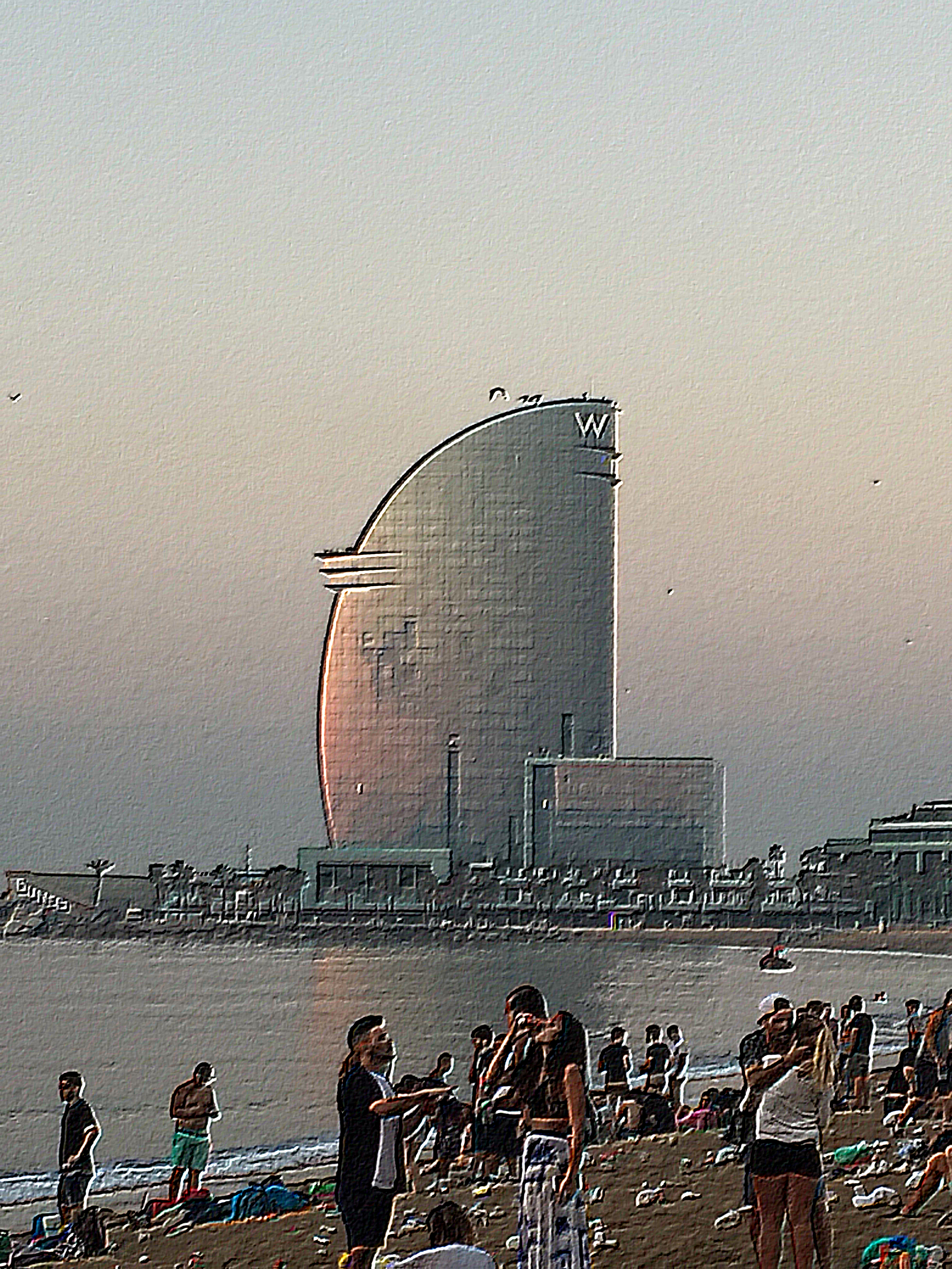
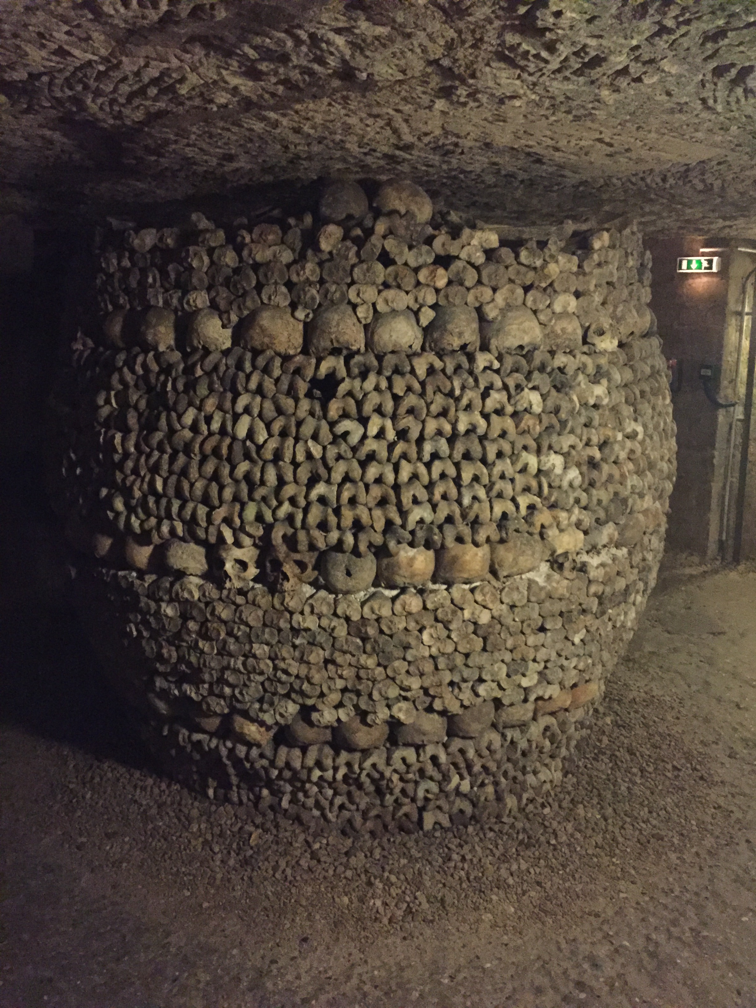
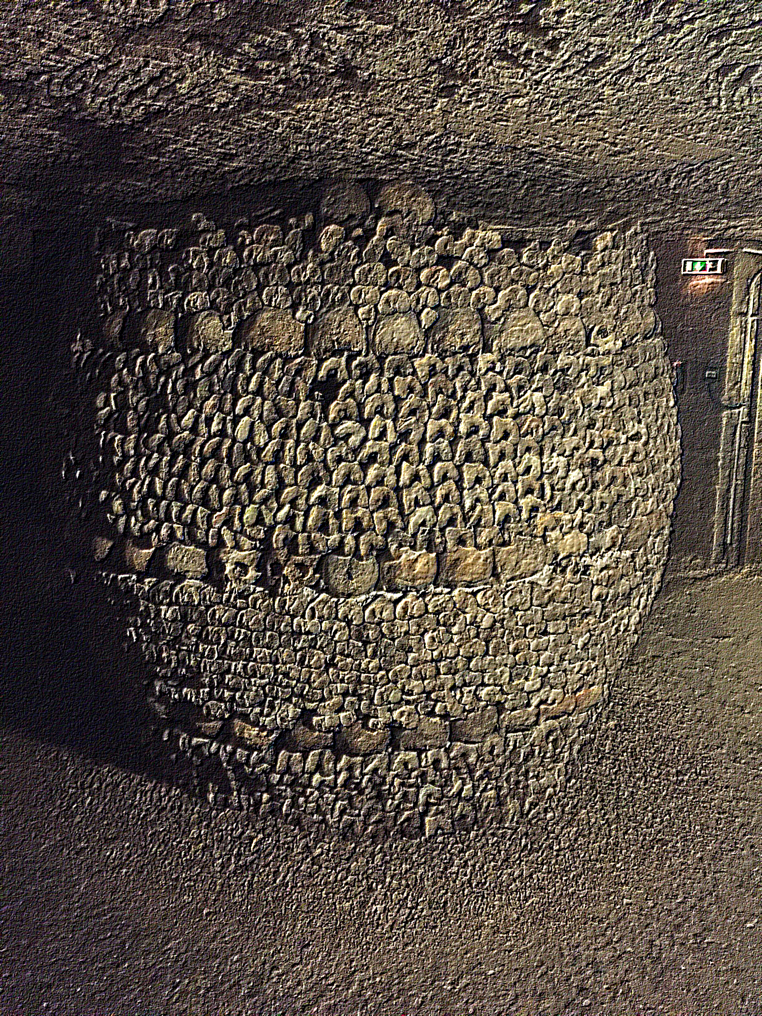
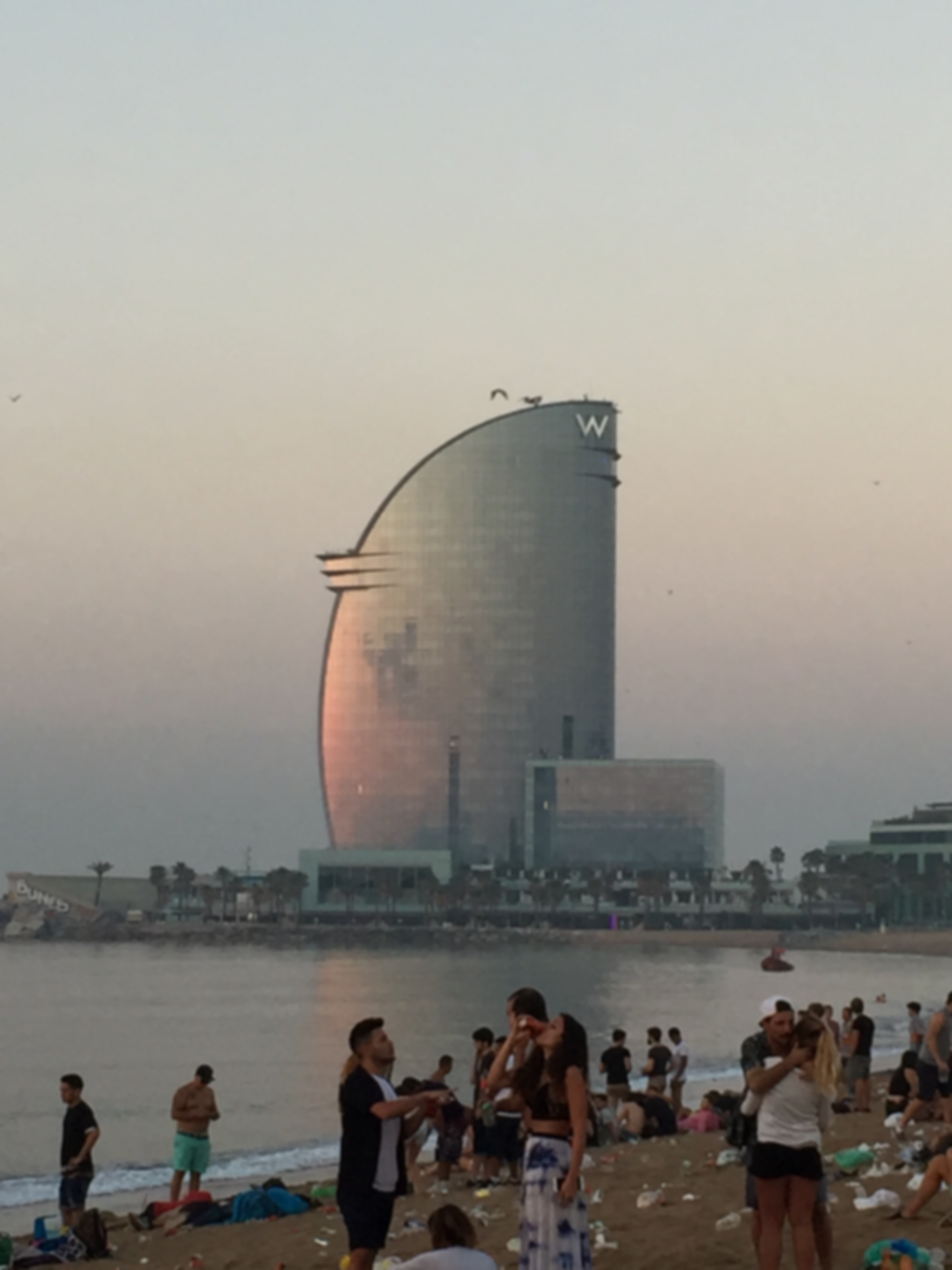
Embossing: (a) original image; (b) embossed image (kernel_size = 5) Embossing: (a) original image; (b) embossed image (kernel_size = 5) Embossing: (a) original image; (b) embossed image (kernel_size = 5)Figures 10{reference-type="ref" reference="fig:emboss_hotel_vela"}, 11{reference-type="ref" reference="fig:emboss_bce"} and 12{reference-type="ref" reference="fig:emboss_catacumbas"} show the results of this filter. Figure 10{reference-type="ref" reference="fig:emboss_hotel_vela"} creates a rather visually exciting result, as it is the one where the results obtain a most different effect. Figures 11{reference-type="ref" reference="fig:emboss_bce"} and 12{reference-type="ref" reference="fig:emboss_catacumbas"} show results that could be regarded as similar to some extreme sharpening, although the results are pretty different when paying close attention.
This effect is not---to my knowledge---a well-known effect described in the literature, but the result of creatively combining several effects that were programmed during the development of this project to obtain a very different image than the original. Although the initial experiments that led to this filter were intended to achieve a sketch result, the obtained filter does not achieve quite that. This filter has been named after American artist Joseph Yoakum (1891-1972) for how the effects of this filter---in my own opinion---resemble his unusual painting style.
This filter combines bilateral filtering, quantisation, outlining convolution, thresholding, and antialiasing convolution. However, bilateral filtering is only a component of this filter that was added in replacement of others in the latest stages of the project. It is also used in the following sections, with a much more critical role. Therefore, its implementation is not discussed in here but in Section 6.3.
def yoakumization(img, levels, bilateral_size, sigma1, sigma2):

    '''
    Apply a cartoon effect to the image.

    Args:
        img (np.array): An RGB image.
        levels (int): Number of quantization levels.
        bilateral_size (number): Bilateral filter size that will be applied.
        sigma1 (number): Bilateral filter sigma 1 that will be applied.
        sigma2 (number): Bilateral filter sigma 2 that will be applied.

    Return:
        An image after applying the stained glass effect.
    '''

    # Make sure the kernel size is an odd number. Otherwise, make it odd by adding one and print a
    # warning.
    if bilateral_size % 2 == 0:
        bilateral_size += 1
        print_debug('Kernel size must be odd. The value used will be {}'.format(bilateral_size))

    # Apply a bilateral filter to remove textures.
    channels = split_channels(img)
    channels = [bilateral_filter(c, bilateral_size, sigma1, sigma2) for c in channels]
    smooth_image = merge_channels(channels)

    # Get the quantization size.
    step = 255 // levels

    # Apply a quantization filter to the image.
    img_quant = (smooth_image // step) * step

    # Get the outlining kernel.
    kernel = np.array([
        [ 1,  1,  1],
        [ 1, -8,  1],
        [ 1,  1,  1]
    ])
    outlined = convolve_all_channels(img_quant, kernel, True)
    outlined[outlined > 255] = 255
    outlined[outlined < 0] = 0

    # Convert it to black and white cause we only care abut lines themselves.
    outlined = color_rgb_to_gray(outlined).astype('float32')

    # Threshold it.
    outlined[outlined < 10] = 0
    outlined[outlined >= 10] = 0.5

    # Invert it to use it as a mask.
    outlined = 1 - outlined

    # Multiply the outline by the quantization.
    ret_img =  img_quant.astype('float32') * merge_channels((outlined, outlined, outlined))

    # Round it to have proper values.
    ret_img = np.round(ret_img)

    # Convolve it to get a filter to avoid heavy aliasing.
    # Get the outlining kernel.
    kernel = np.array([
        [ 0,  1,  0],
        [ 1,  4,  1],
        [ 0,  1,  0]
    ])
    ret_img = convolve_all_channels(ret_img, kernel, True)
    ret_img = ret_img // np.sum(kernel)

    return ret_img.astype('uint8')
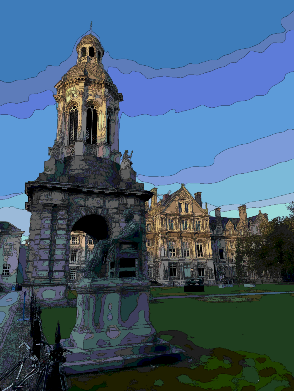
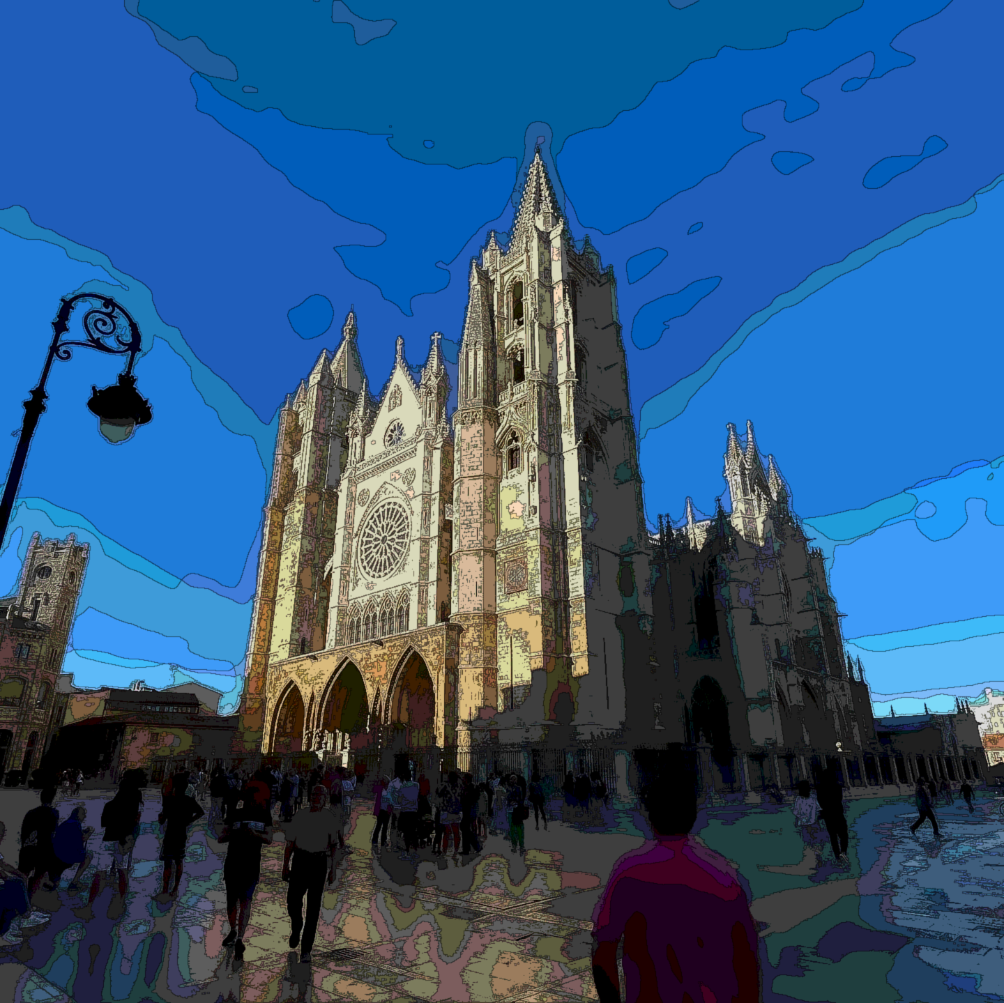
The code above these lines shows the implementation of this unusual filter. First, a bilateral filter is applied to the different channels of the image to obtain an image without texture and with a flat appearance. The resulting colours are then quantisised to obtain homogeneous colour regions that contrast. Next, an outlining convolution is applied to obtain the edges of the colour regions. Next, this image containing the edges is converted to grayscale to obtain a single value for each pixel. Following, it is thresholded so that all the values are either 0 or 0.5. After inverting the values, the quantisised image is multiplied by this new mask. This causes those pixels considered edges to drastically lower their colour without becoming black. Finally, a smooth antialiasing convolution is applied to reduce edge aliasing and give the image a smoother look.
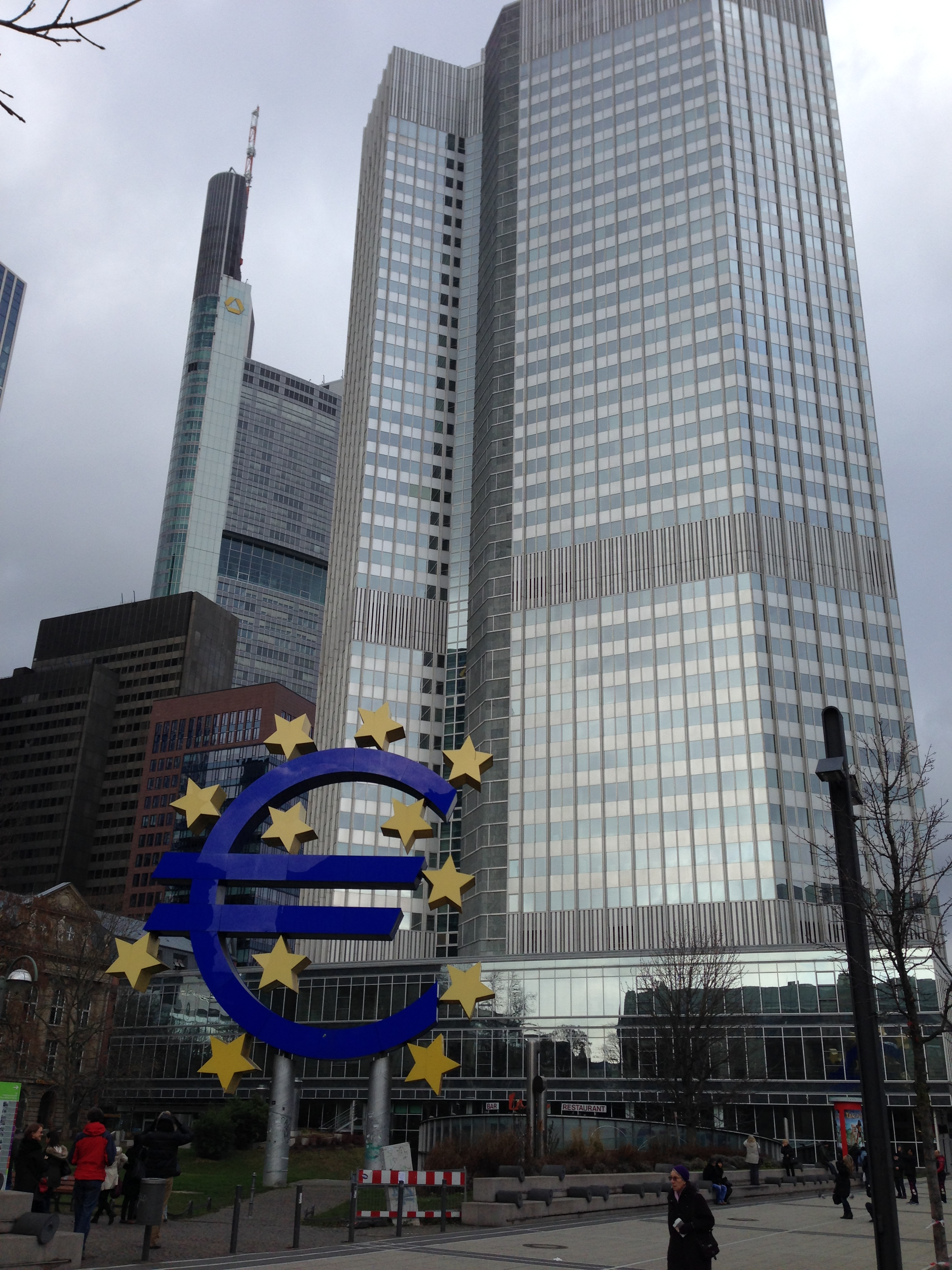
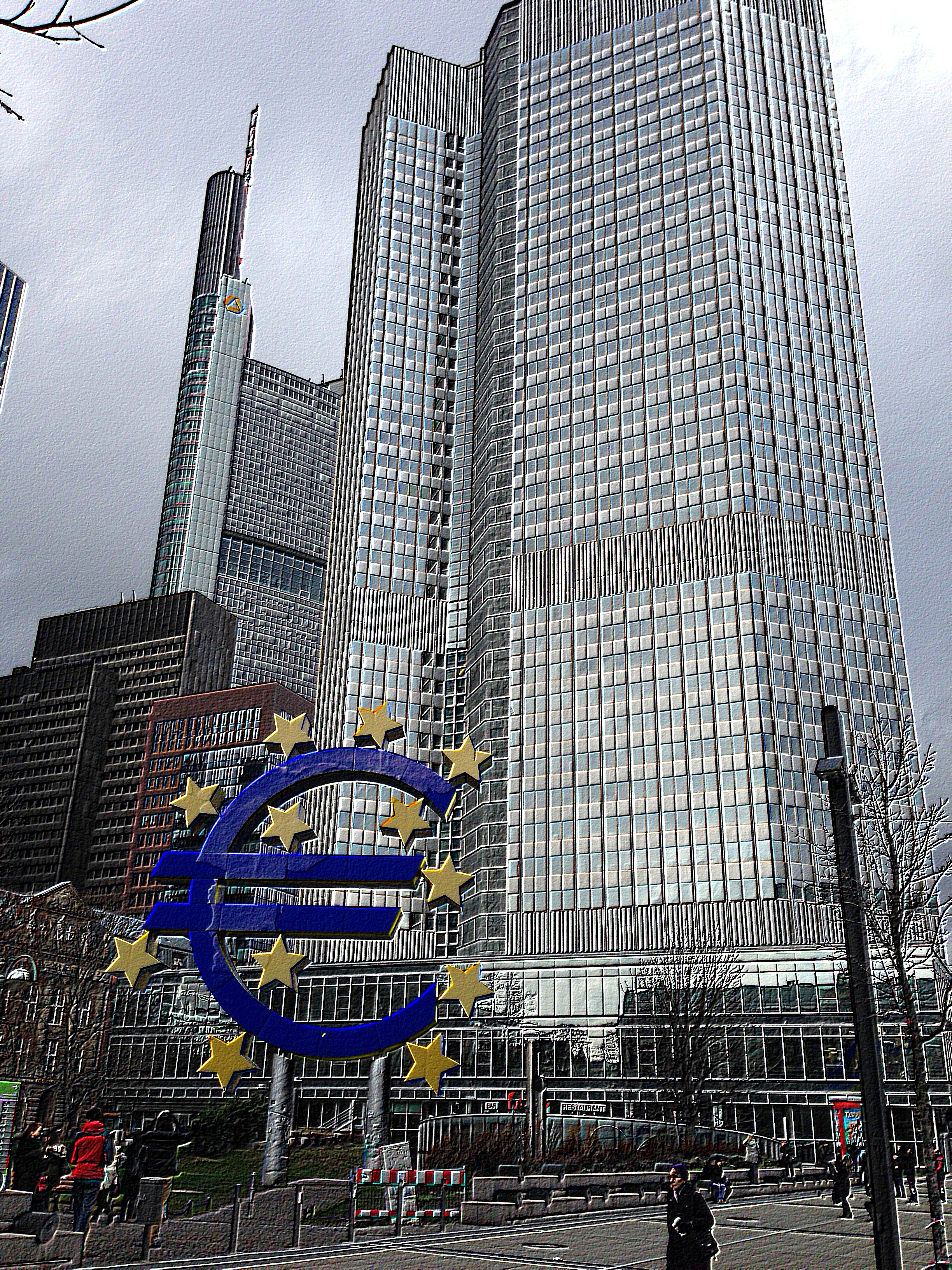
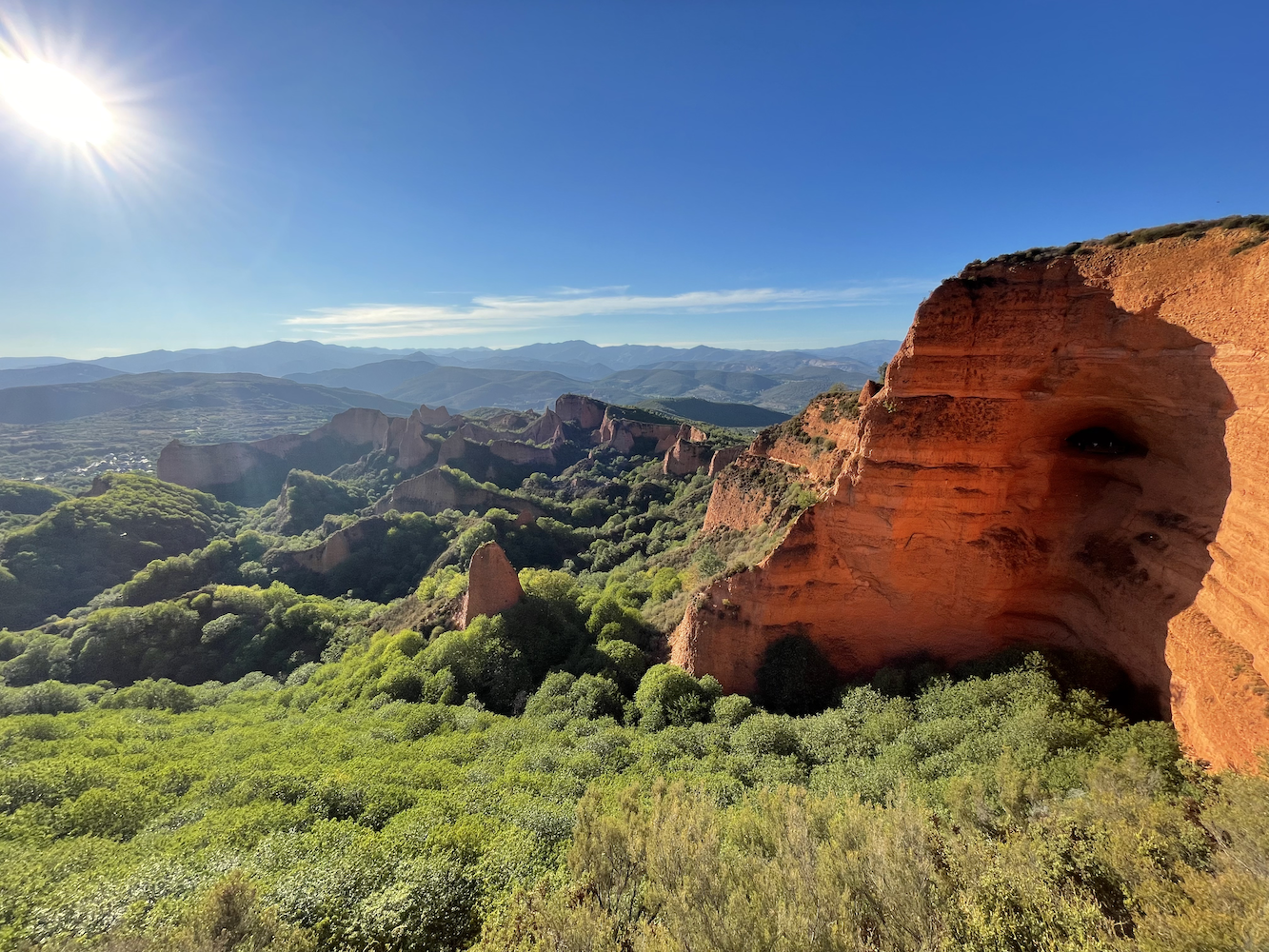
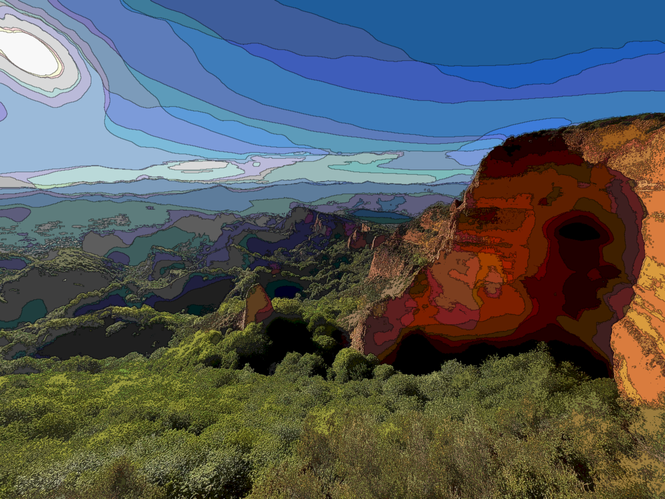
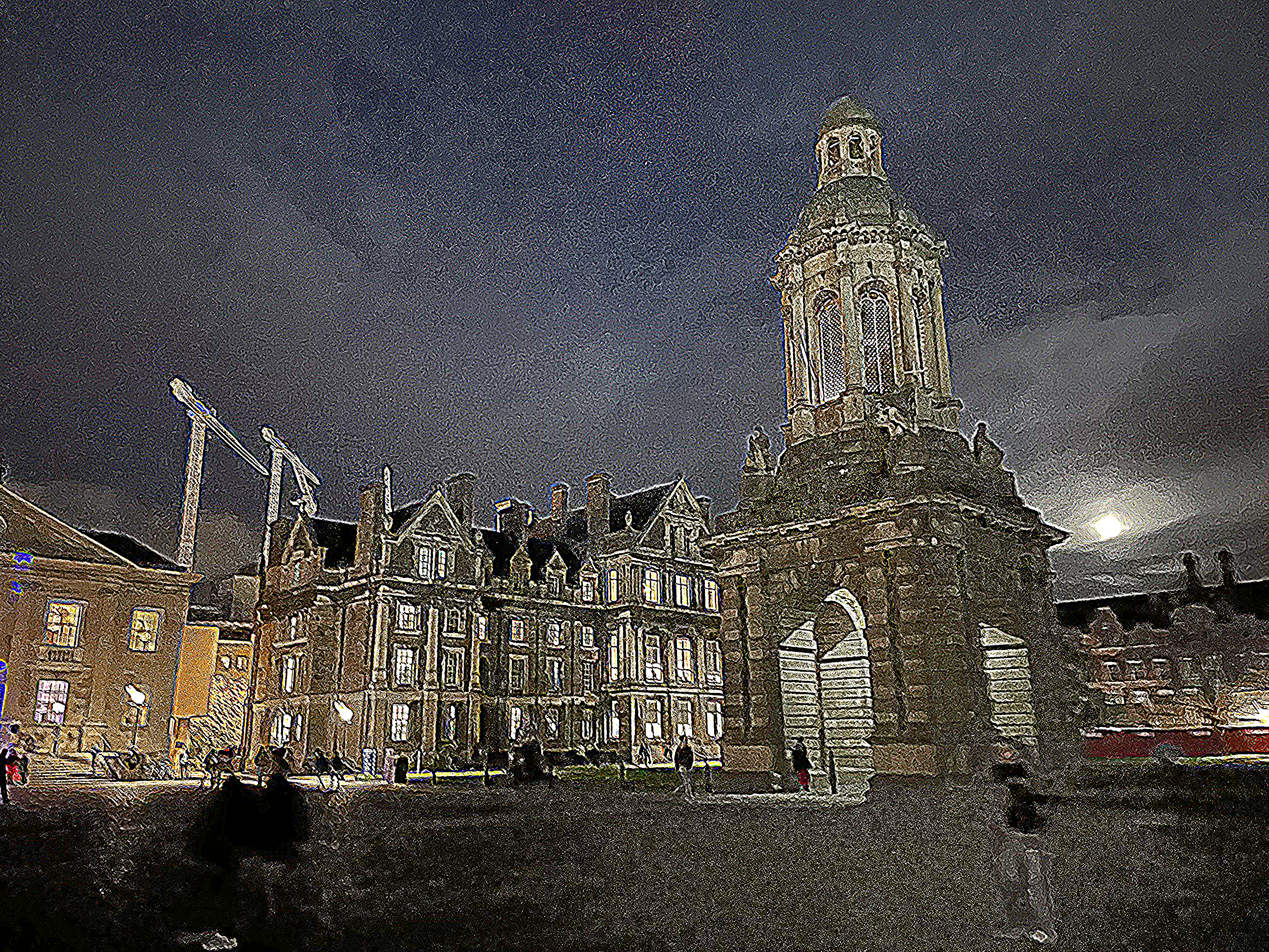
Yoakumisation: (a) original image; (b) Yoakumised image Yoakumisation: (a) original image; (b) Yoakumised image Yoakumisation: (a) original image; (b) Yoakumised imageFigures 13{reference-type="ref" reference="fig:yoakum_medulas_crop"}, 14{reference-type="ref" reference="fig:yoakum_trinity_day_crop"}, and 15{reference-type="ref" reference="fig:yoakum_leon_catedral_exterior"} show the result of applying this filter to the images. The outcome resembles a drawing, although it shows unusual colours and stripes, as well as strongly marked edges in dark colours.
def median_filter(img, kh, kw):

    '''
    Apply a Median blur effect to the image img.

    Args:
        img (np.array): An RGB image.
        kh (int): The to-be-generated kernel height.
        kw (int): The to-be-generated kernel width.

    Return:
        An image after applying the gaussian blur.
    '''

    # Generate the kernel from the specified arguments.
    kernel = np.ones((kh, kw))

    # Convert the image to uint64 to avoid overflows.
    img = img.astype('uint64')

    # Convolve the image using the kernel.
    result_img = convolve_all_channels(img, kernel, True)

    # Normalize the image.
    result_img = result_img // np.sum(kernel)

    return result_img.astype('uint8')
The code above shows the implementation of the median filter in this project. Having described all the functions this method uses, the code is straightforward. First, the kernel is created as a KHxKW matrix of ones. Then this kernel is convolved on the image, and finally, the image is scaled by 1/9---the sum of the kernel cells--- to regain the initial colour range.
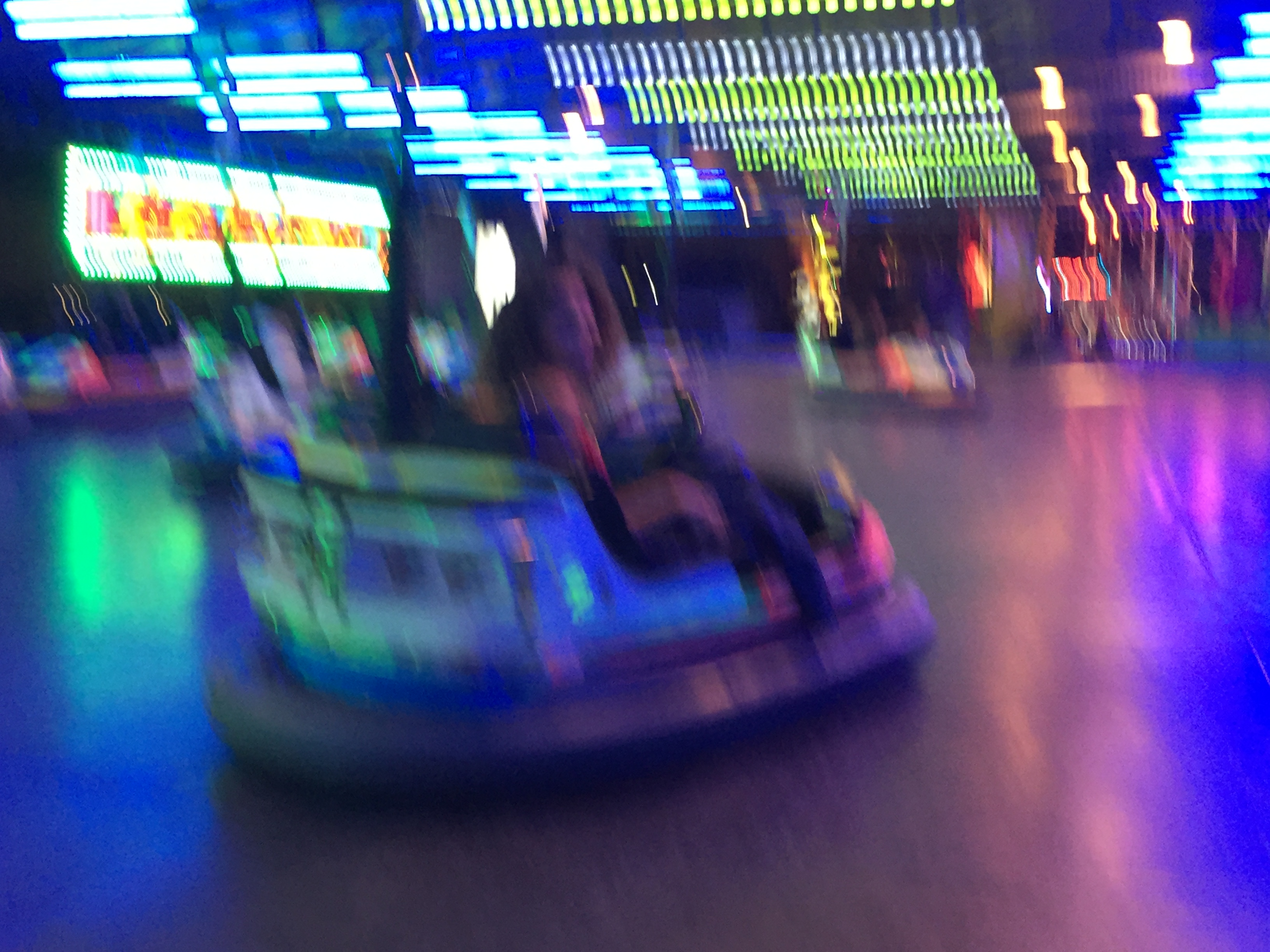
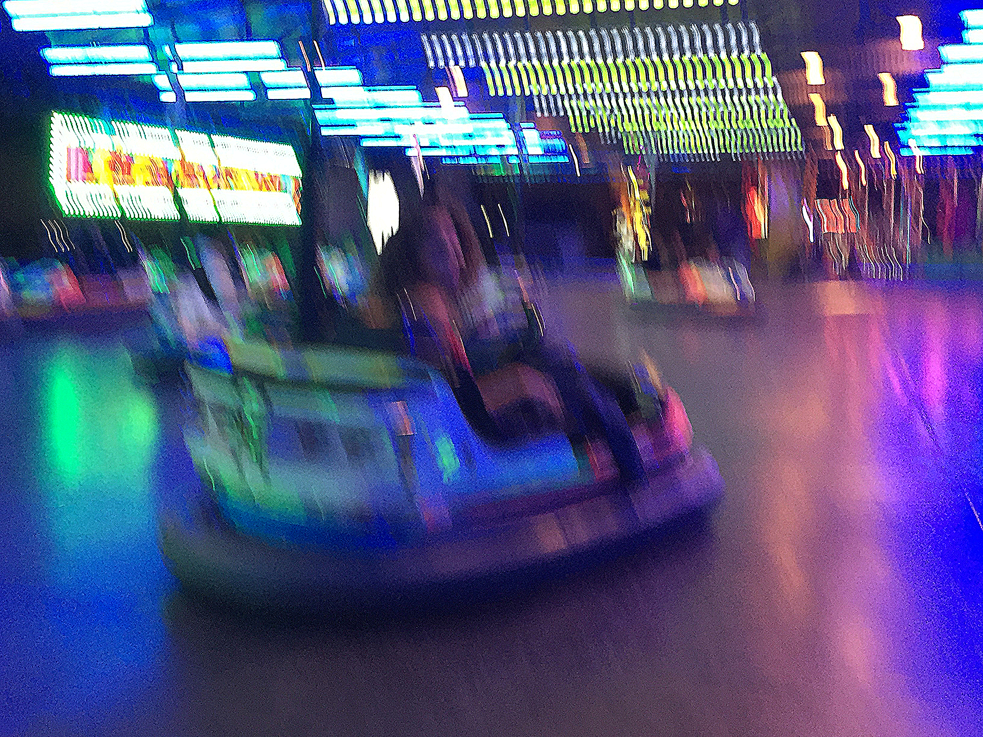
This relatively simple filter can get excellent results when used with small kernels to reduce image noise. Figures A, B and C show the results of applying the median filter to 3 selected noisy pictures. The kernel sizes have been selected considering the shapes and noise found in the images.
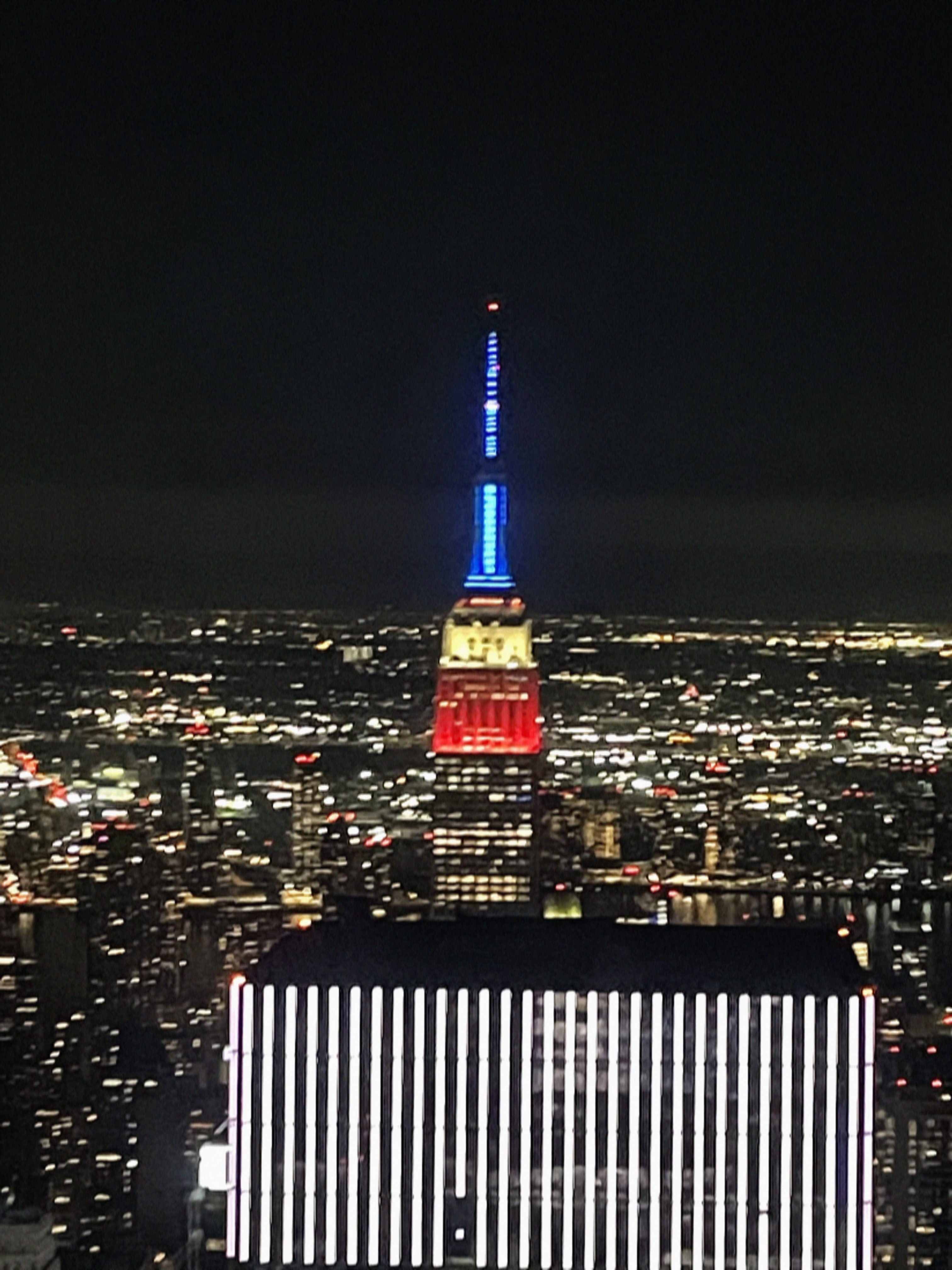
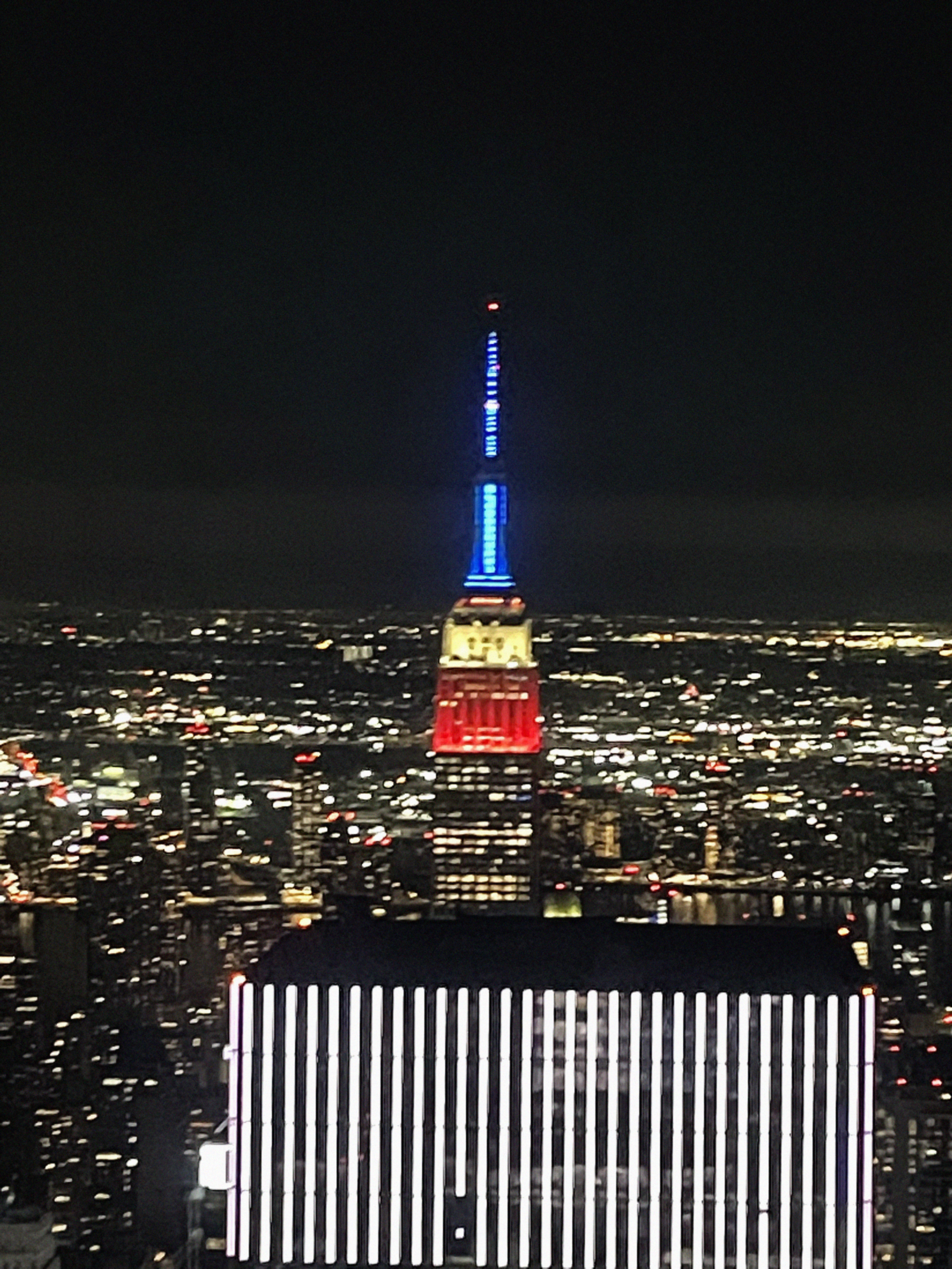
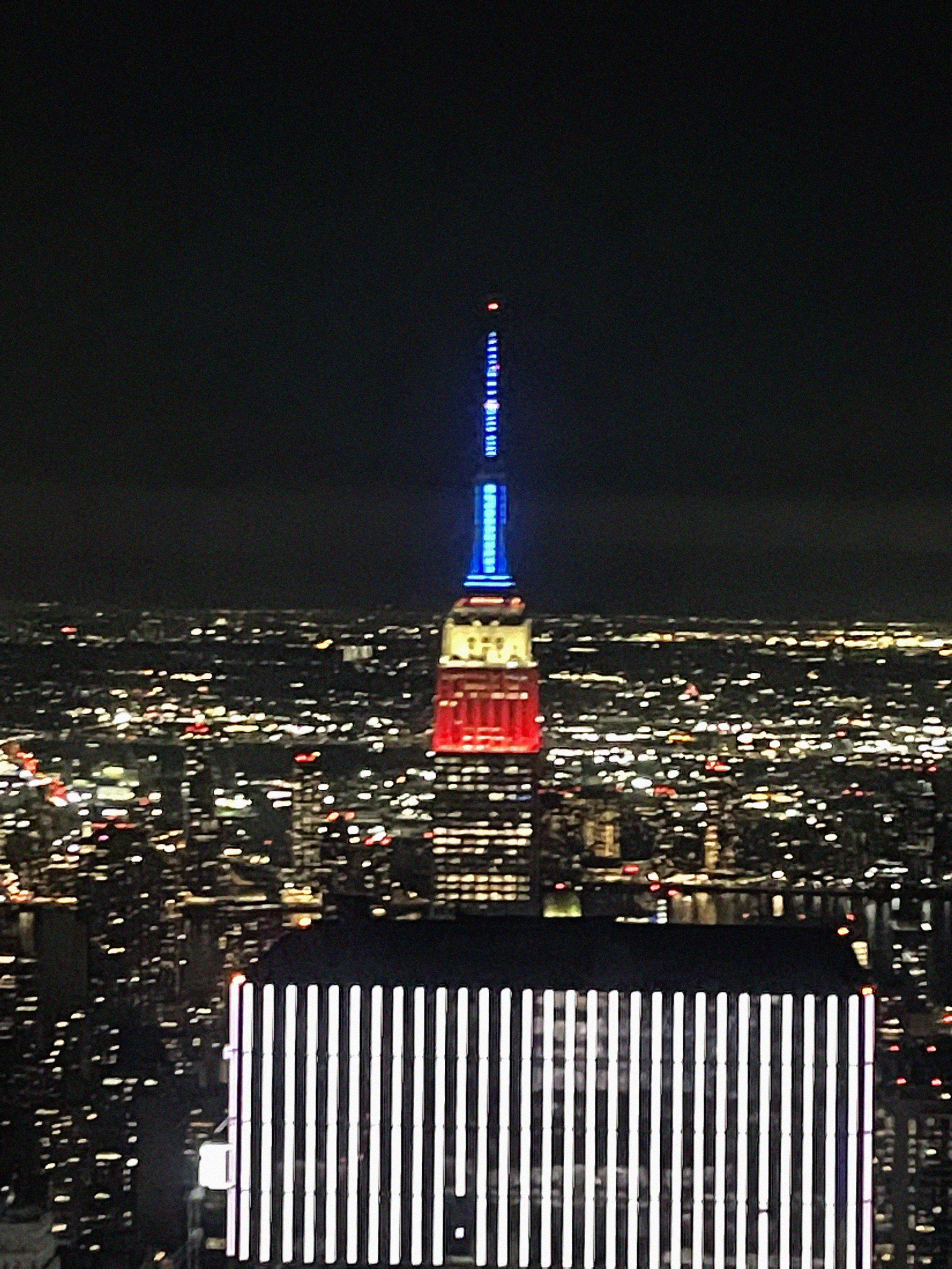
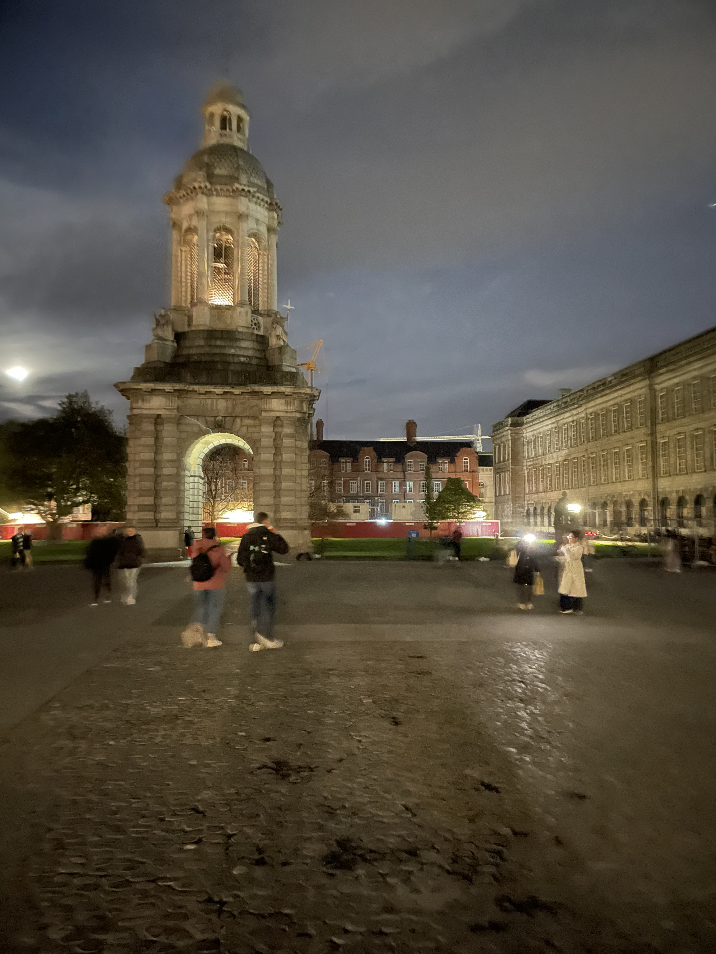
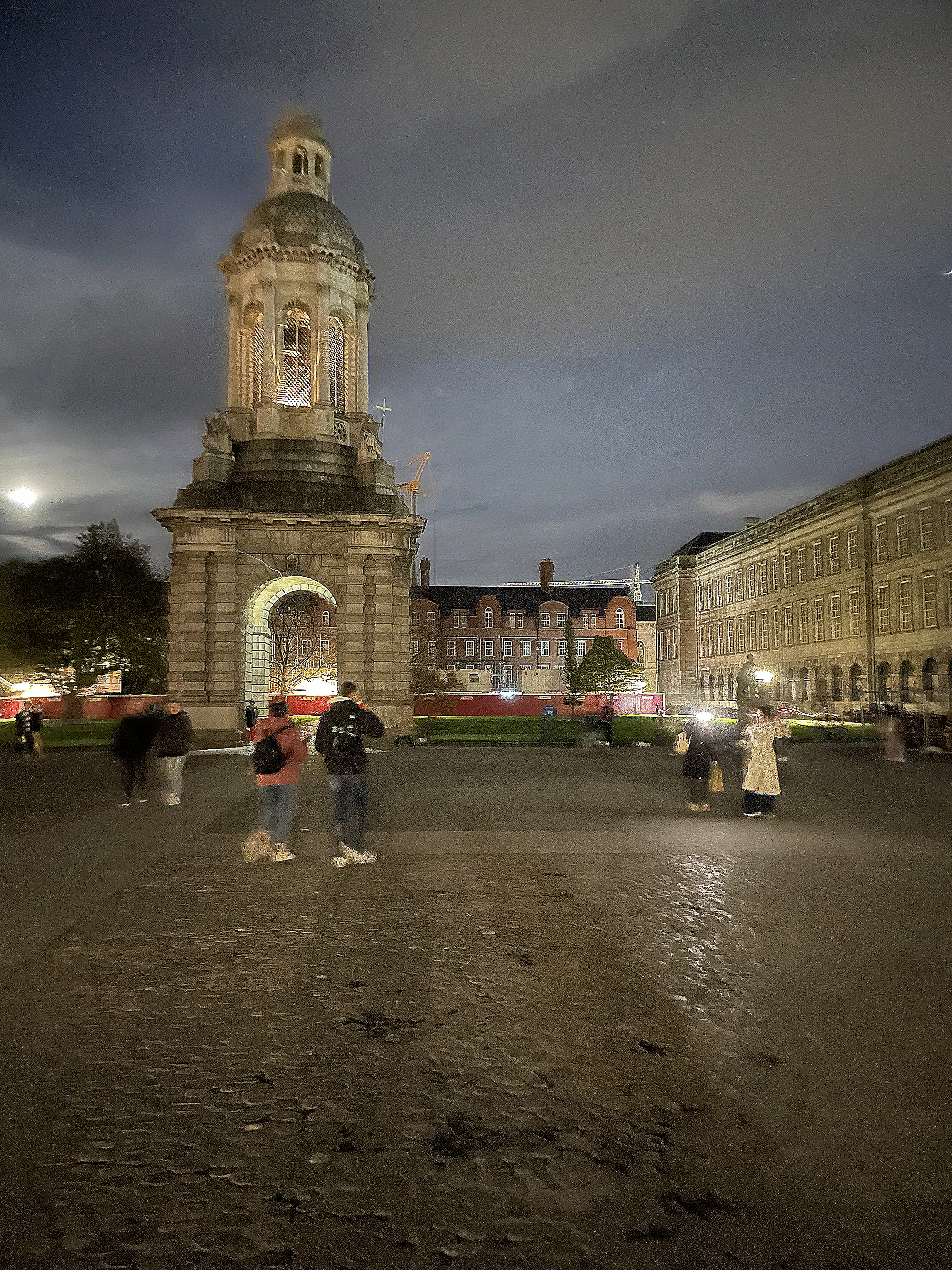
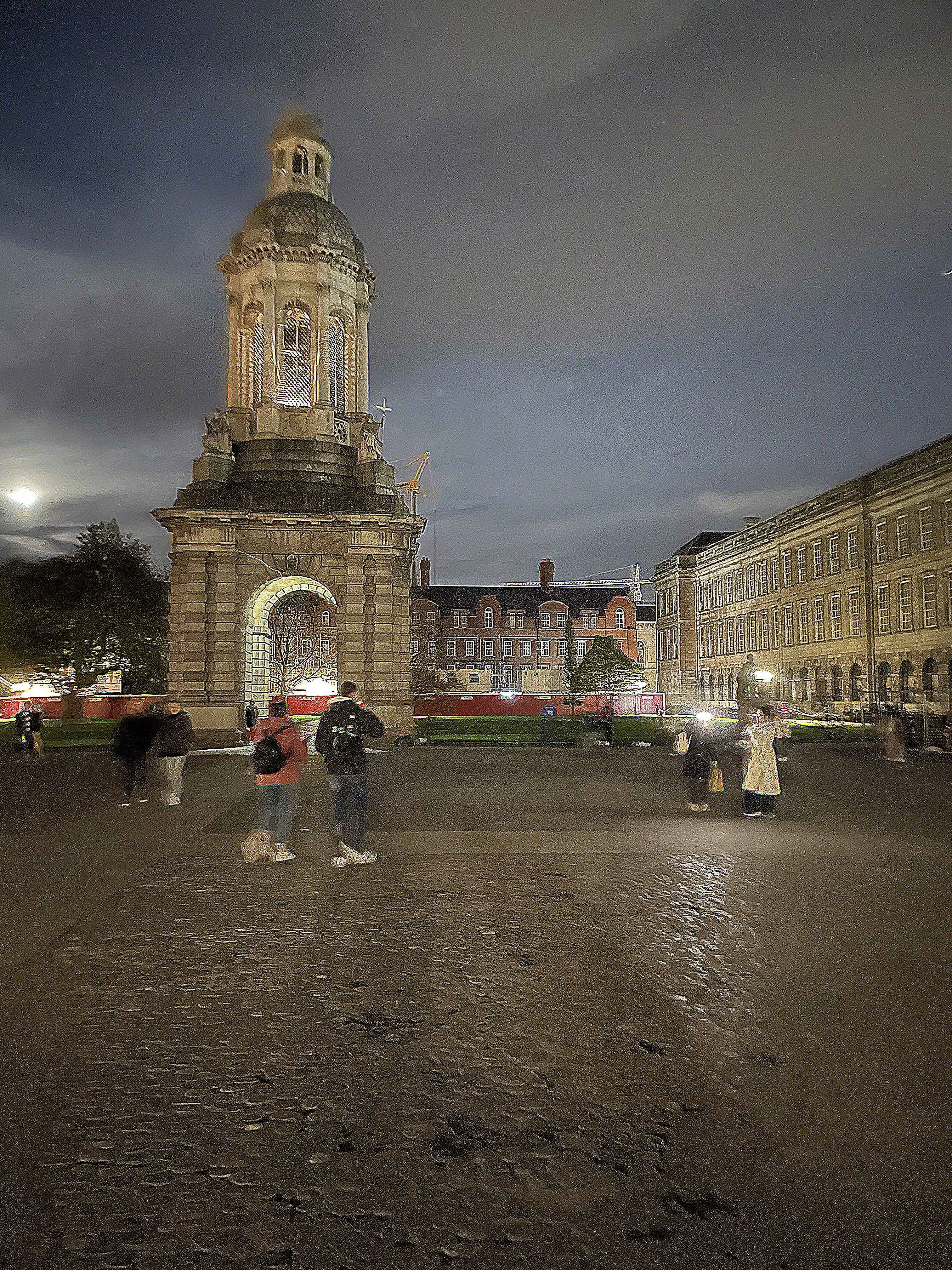
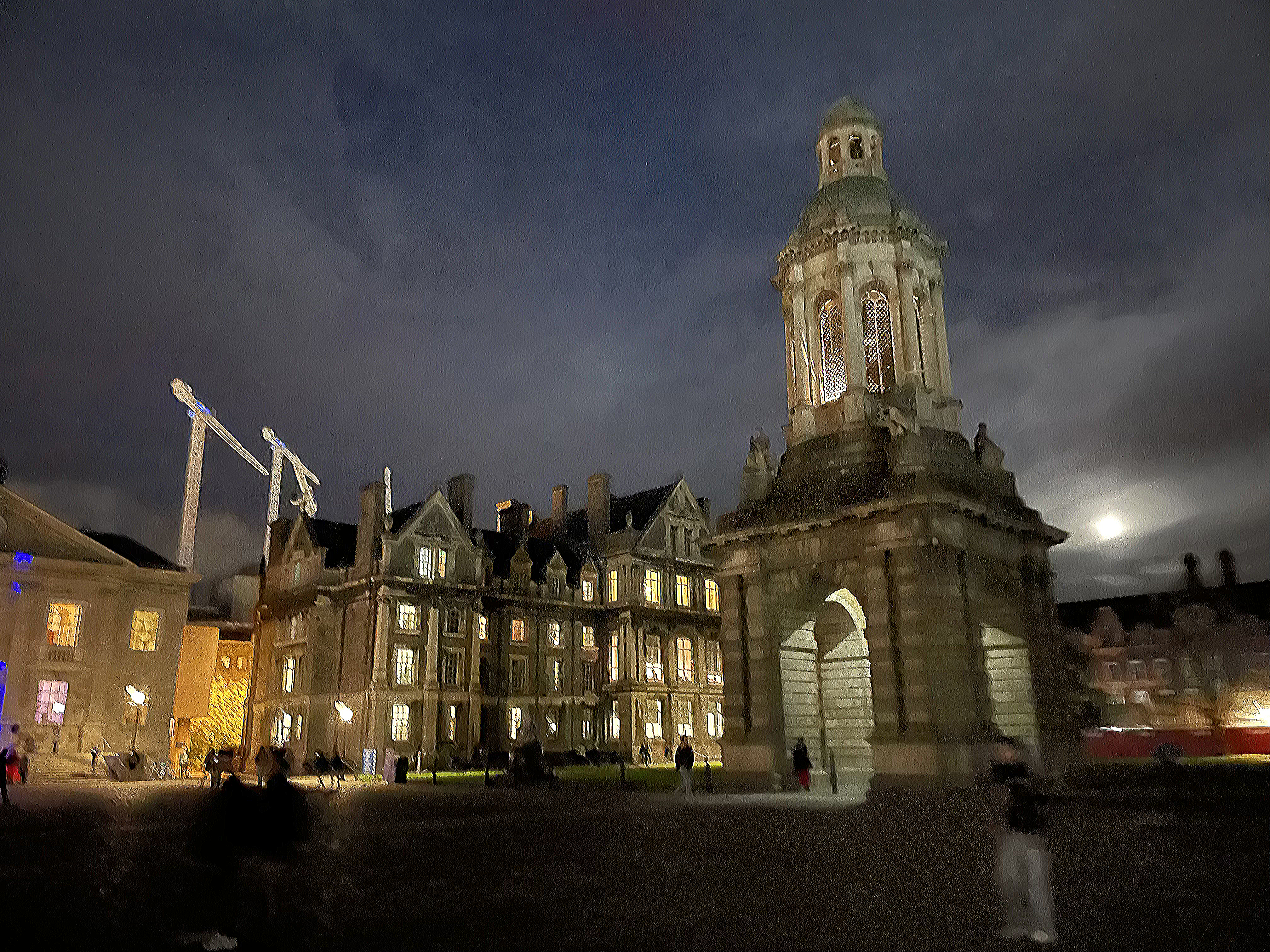
Median filter: (a) original image; (b) median filter (kh = 3, kw = 3) Median filter: (a) original image; (b) median filter (kh = 9, kw = 3) Median filter: (a) original image; (b) median filter (kh = 7, kw = 7)Figure 16{reference-type="ref" reference="fig:median_trinity_noche"} shows little improvement due to the kind of noise found in the image. The noise does not limit to pixels with high colour variation but is composed of more extensive areas of patches with artefacts caused by the camera's night mode. Therefore, when applying a kernel large enough to manage this kind of noise, the image becomes too blurry.
Figure 17{reference-type="ref" reference="fig:median_empire_state_bad"} shows the best results of the three images. The original image contains two problems: it is noticeably blurry, and it contains very sharp noise. This combination is due to the fact that it is a scanned copy of a blurred photo. A significant noise reduction is achieved by applying a mostly vertical kernel to this image---desirable because of the shape of the main objects. Although it also introduces blur, this fact is concealed by the blur the photo initially contained.
Figure 18{reference-type="ref" reference="fig:median_hotel_vela"} shows a significant reduction in noise in clear areas, despite losing sharpness in sharp contrast areas. However, removing the most noticeable noise artefacts is only possible by making the image very blurry.
def gaussian_func(x, y, sigma):

    '''
    Calculate the gaussian function for given X, Y and sigma values.

    Args:
        x (number): X variable of the gaussian function.
        y (number): Y variable of the gaussian function.
        sigma (number): Sigma constant.

    Return:
        The result of the gaussian function.
    '''

    # Split the formula in two to make it readable.
    gauss1 = 1 / (2 * np.pi * sigma ** 2)
    gauss2 = np.exp(-(x ** 2 + y ** 2) / (2 * sigma ** 2))

    return gauss1 * gauss2

def gaussian_blur(img, kh, kw, sigma):

    '''
    Apply a Gaussian blur effect to the image img.

    Args:
        img (np.array): An RGB image.
        kh (int): The to-be-generated kernel height.
        kw (int): The to-be-generated kernel width.
        sigma (number): Sigma constant.

    Return:
        An image after applying the gaussian blur.
    '''

    # Generate the gaussian kernel from the specified arguments.
    gauss_y, gauss_x = np.indices((kh, kw), dtype='float64')
    gauss_y -= kh // 2
    gauss_x -= kw // 2
    kernel = gaussian_func(gauss_x, gauss_y, sigma)

    # Normalize the kernel to integers.
    # kernel = (kernel // np.min(kernel)).astype('uint64')

    # Convert the image to uint64 to avoid overflows.
    img = img.astype('float64')

    # Convolve the image using the kernel.
    result_img = convolve_all_channels(img, kernel, True)

    # Normalize the image.
    result_img = result_img // np.sum(kernel)

    return result_img.astype('uint8')
The code above shows the implementation of the Gaussian blur filter in this project. Function gaussian_func implements the Gaussian function, defined on its 1 and 2 dimensions as:
The function implemented in this project is done using NumPy and allows to make the calculations in parallel for big sets of X and Y values.
Function Gaussian_blur implements the filter itself. The kernel height, width, and sigma values are the only parameters in this function. Therefore, the first task in the function is to build the Gaussian kernel. First, NumPy's indices method obtains the X and Y indices of the matrix's cells as matrices. Next, these matrices are normalised around its centre---making the index on the centre (0,0). Then vertical and horizontal indexes are fed to the gaussian_func matrix to obtain the value for each cell. Finally, this kernel is used to convolve the image, and the image is normalised before returning it.
Gaussian blur: (a) original image; (b) kh = 5, kw = 5, σ = 1; (c) kh = 5, kw = 5, σ = 5; (d) kh = 10, kw = 10, σ = 0.5. Gaussian blur: (a) original image; (b) kh = 5, kw = 5, σ = 1; (c) kh = 5, kw = 5, σ = 5; (d) kh = 10, kw = 10, σ = 0.5. Gaussian blur: (a) original image; (b) kh = 5, kw = 5, σ = 1; (c) kh = 5, kw = 5, σ = 5; (d) kh = 10, kw = 10, σ = 0.5.Gaussian blur is much more delicate when dealing with image noise than other filters. It achieves results with a more continuous appearance than the median filter without having to give up the sharpness of the objects in return.
Figures 19{reference-type="ref"
reference="fig:gaussian_blur_trinity_noche"} and
21{reference-type="ref"
reference="fig:gaussian_blur_hotel_vela"} show a much more blended noise
in the image, with smooth surfaces with a more continuous appearance
than the median filter. However, in both cases, the 10x10 size with
In Figure 20{reference-type="ref" reference="fig:gaussian_blur_empire_state_bad"}, it can be seen that the background noise has not entirely disappeared but has become a haze that slightly modifies the colour of the background. Although it is better to have an integrated background, the median filter will probably work better for this type of high-concentration noise.
def bilateral_filter(img, kernel_size, sig_r, sig_s):

    '''
    Implements a bilateral filter.

    Args:
        img (np.array): An RGB image.
        kernel_size (number): Size of the kernel that will be used to compute the convolution.
        sig_r (number): Sigma constant of the gaussian function f_r.
        sig_s (number): Sigma constant of the gaussian function g_s.

    Returns:
        The resulting image after applying the convolution.

    See:
        https://en.wikipedia.org/wiki/Bilateral_filter
    '''

    # Make sure the kernel size is an odd number. Otherwise, make it odd by adding one and print a
    # warning.
    if kernel_size % 2 == 0:
        kernel_size += 1
        print_debug('Kernel size must be odd. The value used will be {}'.format(kernel_size))

    # Convert the image to int64 to avoid clipping problems.
    img = img.astype(np.int64)

    # Get a copy of the image that will be used as the original image.
    org_img = img.copy()

    # Pad the image to avoid errors.
    # To do this we use half the size of the kernel, as it is the further away it'll go.
    img = np.pad(img, pad_width=kernel_size // 2, mode='edge')

    # Get the image dimensions.
    img_height = img.shape[0]
    img_width = img.shape[1]

    # Get the convolved image sizes.
    conv_height = img_height - (kernel_size - 1)
    conv_width = img_width - (kernel_size - 1)

    # Init the resulting image.
    result = np.zeros((conv_height, conv_width))

    # Init the W_p normalizer accumulator.
    w_p = 0

    # Iterate through the kernel cells.
    for x in range(kernel_size):
        for y in range(kernel_size):

            # Get the end index.
            # This is the index next to the last one we want to get.
            end_y = img_height - (kernel_size - y) + 1
            end_x = img_width - (kernel_size - x) + 1

            # Get the current submatrix.
            submatrix = img[y:end_y, x:end_x]

            # Get the two matrix components from the bilateral function.
            f_r = gaussian_func(submatrix - org_img, 0, sig_r)
            g_s = gaussian_func(euclidian(np.array([x, y]),
                    np.array([kernel_size // 2, kernel_size // 2])), 0, sig_s)

            # Calculate the W_p normalizer.
            modifier = f_r * g_s

            # Apply the kernel and spatial and modifiers.
            result = result + (submatrix * modifier)

            # Apply the W_p summatory.
            w_p += modifier

    # Normalize the image.
    result = result // w_p

    return result.astype('uint8')
The code below these lines implements the bilateral filter. This code is, in its structure, very similar to a regular convolution. The difference is that a typical convolution uses the pixel and the kernel cell to compute the result, but the bilateral filter does more than that. The bilateral filter calculates the final value using two Gaussian functions operating on the value of the cells, the value of neighbouring cells, and the Euclidean distance between their coordinates and the centre of the kernel. This allows the filter to modulate the blur with distance (like Gaussian blur) and colour difference.
The code above shows how the function extracts a complete sub-matrix for each kernel cell. Then, this matrix and the original image are input to one of the Gaussian functions. At the same time, the coordinate difference is passed to another Gaussian function to modulate the output. Finally, the resulting matrix is normalised and returned.
Bilateral filter: (a) original image; (b) size = 5, σr = 5.0, σs = 1.0; (c) size = 5, σr = 1.0, σs = 5.0; (d) size = 21, σr = 20.0, σs = 10.0. Bilateral filter: (a) original image; (b) size = 5, σr = 5.0, σs = 1.0; (c) size = 5, σr = 1.0, σs = 5.0; (d) size = 21, σr = 20.0, σs = 10.0. Bilateral filter: (a) original image; (b) size = 5, σr = 5.0, σs = 1.0; (c) size = 5, σr = 1.0, σs = 5.0; (d) size = 21, σr = 20.0, σs = 10.0.In Figures
22{reference-type="ref"
reference="fig:bilateral_filter_trinity_noche"} and
24{reference-type="ref"
reference="fig:bilateral_filter_hotel_vela"}, size = 5 with
On the other hand, when it comes to larger kernel sizes and higher
In the case of Figure 23{reference-type="ref" reference="fig:bilateral_filter_empire_state_bad"}, this is not a filter that gets any improvement. Lower values leave the image noise unchanged due to its high contrast. On the other hand, higher parameter values lead to gains similar to Gaussian blur with much more significant losses.
def bartlett_filter(img, kernel_size):

    '''
    Applies a Bartlett filter to all channels.

    Args:
        img (np.array): An RGB image.
        kernel_size (number): Size of the kernel that will be used to compute the convolution.

    Returns:
        The resulting image after applying the convolution.

    See:
        https://research.cs.wisc.edu/graphics/Courses/559-f2002/lectures/cs559-7.ppt
    '''

    # Make sure the kernel size is an odd number. Otherwise, make it odd by adding one and print a
    # warning.
    if kernel_size % 2 == 0:
        kernel_size += 1
        print_debug('Kernel size must be odd. The value used will be {}'.format(kernel_size))

    # Get the kernel central index.
    kernel_center = kernel_size // 2

    # Get the generators for the kernel. The kernel will be the result of multiplying both arrays.
    kernel_gen = [(kernel_center + 1) - abs(i - kernel_center) for i in range(kernel_size)]
    kernel_gen_1 = np.array([kernel_gen for i in range(kernel_size)])
    kernel_gen_2 = np.transpose(kernel_gen_1)

    # Get the final kernel.
    kernel = kernel_gen_1 * kernel_gen_2

    # Convolve all channels using this kernel.
    ret_img = convolve_all_channels(img.astype('uint64'), kernel, True)

    # Normalize the image.
    ret_img = ret_img // np.sum(kernel)

    return ret_img.astype('uint8')
The Bartlett's filter is a convolution filter for which a linear tent kernel is used. To implement this filter, the kernel is created by multiplying a 1D tent kernel with its transposed matrix. In the code above, the matrix multiplication is done by replicating the columns or rows and doing a cell-by-cell multiplication. This kernel is then used to convolve the image, and the result is returned after normalised.
This filter obtains a kernel that gives more weight to the pixels closest to the centre of the kernel. Unlike Gaussian blur, this weight evolves linearly.
Bartlett’s filter: (a) original image; (b) size = 5; (c) size = 9; (d) size = 15. Bartlett’s filter: (a) original image; (b) size = 5; (c) size = 9; (d) size = 15. Bartlett’s filter: (a) original image; (b) size = 5; (c) size = 9; (d) size = 15.Figure 25{reference-type="ref" reference="fig:bartlett_trinity_noche"}, 26{reference-type="ref" reference="fig:bartlett_empire_state_bad"}, and 27{reference-type="ref" reference="fig:bartlett_hotel_vela"} can give us a fascinating inside look at the logic of how kernels affect images when they are compared to those in Gaussian blur and Median filter. This filter gets results that are in the middle of both filters. While Bartlett's filter does give bigger weights to the central kernels, the weight of farther ones is not as low. Therefore, it offers a trade-off between the pros and cons of each filter that is worth considering.
Figure 26{reference-type="ref" reference="fig:bartlett_empire_state_bad"} shows the silver linings of this filter. Bartlett's filter achieves a better result at correcting the noise of this image, as it does not cause such heavy background changes while achieving a smooth result.
def unsharp_mask(img, kw, kh):

    '''
    Applies a Unsharp masking sharpening effect on all channels.

    Args:
        img (np.array): An RGB image.
        kh (int): The to-be-generated kernel height.
        kw (int): The to-be-generated kernel width.

    Returns:
        The resulting image after applying the convolution.

    See:
        https://homepages.inf.ed.ac.uk/rbf/HIPR2/unsharp.htm
        https://en.wikipedia.org/wiki/Unsharp_masking
    '''

    # Generate the kernel.

    # The unsharp masking kernel is the result of operating with two kernels: the 'cross' and the
    # identity kernel.

    # Get the kernel indexes we will use to operate.
    ind_y, ind_x = np.indices((kh, kw), dtype='float64')

    # Get the identity and cross kernels.
    identity_kernel = np.zeros((kh, kw))
    identity_kernel[np.logical_and(ind_y == kh //2, ind_x == kw // 2)] = 1

    cross_kernel = np.zeros((kh, kw))
    cross_kernel[np.logical_or(ind_y == kh //2, ind_x == kw // 2)] = 1

    # Get the desired kernel by operating with these.
    cross_sum = np.sum(cross_kernel)
    kernel = identity_kernel + (identity_kernel - cross_kernel / cross_sum) * cross_sum
    kernel = np.round(kernel).astype('int8')

    # Convolve all channels using this kernel.
    ret_image = convolve_all_channels(img.astype('int64'), kernel, True)

    # Clip the image.
    ret_image[ret_image > 255] = 255
    ret_image[ret_image < 0] = 0

    return ret_image.astype('uint8')
The kernel for this convolution filter is expressed by a simple mathematical expression (Wikipedia), University of Edinburgh):
This expression can be generalised to use bigger identity and cross matrices by changing the scaling number. That is what the code above does to build this filter. It creates an identity and cross matrices of the desired size, then it calculates the new scaling number and performs the operation. This kernel is then used to convolve the image and the result is clipped and returned.
Unsharp mask: (a) original image; (b) size = 5x5; (c) size = 7x7; (d) size = 7x3; (e) size = 3x7; (f) size = 15x15; Unsharp mask: (a) original image; (b) size = 5x5; (c) size = 7x7; (d) size = 7x3; (e) size = 3x7; (f) size = 15x15; Unsharp mask: (a) original image; (b) size = 5x5; (c) size = 7x7; (d) size = 7x3; (e) size = 3x7; (f) size = 15x15;Figures 28{reference-type="ref" reference="fig:unsharp_trinity_noche_movida"} and 29{reference-type="ref" reference="fig:unsharp_trinity_noche_movida_2"} show a reasonably expected behaviour of this filter. In both cases, this filter provides a sensation of greater sharpness in the image. As the kernel size increases, more detail in the image seems to appear. However, 15x15 kernels are, in both cases, too large for the job and fill the image with unnecessary noise.
Figure 30{reference-type="ref" reference="fig:unsharp_auto_de_choque"} shows us an image with a massive blur. In these cases, it can be seen that the unsharp mask acts on the image but does not allow any valuable detail to be enhanced. The 15x15 kernel gives the image a duplicate image effect in this case. It could lead to thinking there is less blur than before, but it does not give us more detail.
def decimate(img, keep_every):

    '''
    Decimate an image by only keeping one every keep_every rows and columns of the original image.

    Args:
        img (np.array): The original image to resample.
        keep_every (int): The number that will be used to determine what cells to keep.

    Return:
        The image after dropping the unwanted columns and rows.
    '''

    # Do it for every channel if it is multi-channel.
    if len(img.shape) == 3:

        # Split the channels, recursively to it and return the combination.
        channels = split_channels(img)
        dec_channels = [decimate(ch, keep_every) for ch in channels]
        return merge_channels(dec_channels)

    # Get the original shape of the image and tranform it into the desired shape.
    shape = list(img.shape)
    shape[0] = shape[0] // keep_every
    shape[1] = shape[1] // keep_every

    # Directly drop excess to avoid numpy complaints.
    img = img[0:shape[0] * keep_every, 0:shape[1] * keep_every]

    # Create an empty matrix of the desired shape.
    # We will use this to repeat the original contents of the image n times.
    img_dec = np.zeros(shape, dtype=img.dtype)

    # Get the indices of the image. This will allow us to operate with the assignation.
    ind_y, ind_x = np.indices((img.shape[0], img.shape[1]), dtype='uint64')

    img_dec[img_dec == 0] = img[np.logical_and(ind_y % keep_every == 0, ind_x % keep_every == 0)]

    return img_dec

def upscale(img, repeat):

    '''
    Upscale the image by repeating n-times each row and column.

    Args:
        img (np.array): The original image to resample.
        keep_every (int): The number that will be used to determine how many times the rows /
                columns will be repeated.

    Return:
        The image after repeating the rows and columns.
    '''

    # Do it for every channel if it is multi-channel.
    if len(img.shape) == 3:

        # Split the channels, recursively to it and return the combination.
        channels = split_channels(img)
        up_channels = [upscale(ch, repeat) for ch in channels]
        return merge_channels(up_channels)

    # Get the original shape of the image and tranform it into the desired shape.
    shape = list(img.shape)
    shape[0] *= repeat
    shape[1] *= repeat

    # Create an empty matrix of the desired shape.
    # We will use this to repeat the original contents of the image n times.
    img_upscaled = np.zeros(shape, dtype=img.dtype)

    # Get the indices of the matrix. This will allow us to operate with the assignation.
    ind_y, ind_x = np.indices((shape[0], shape[1]))

    # We will iterate to get each subcell in the NxN squares of repetition.
    # Finally, assign the values of the image to all the corresponding cells.
    for y in range(repeat):
        for x in range(repeat):

            img_upscaled[np.logical_and(ind_y % repeat == y, ind_x % repeat == x)] = img.flatten()

    return img_upscaled
Resampling (upscaling and decimation) consists of applying interpolation filters and adding new or discarding cells. Different interpolation techniques are used in each of the resampling filters implemented in this project, but the upscaling and decimation functions are the same. These features are described in this section because this is the first time they have appeared in the project. However, they are used in all subsubsections of this section.
Above these lines are the decimate and upscale functions. In the first of these two, a new image of the size of the selected image is created. Then, using NumPy, all those values whose indices have mod N == 0 (being N the ratio of cells to keep) are assigned to the new image. This selects only 1 out of N rows and columns at practical levels.
In the upscale function, a similar mechanism is used, but in reverse.
This time, an image of the desired size is created---larger than the
original. Then, the values of the original image are assigned to the new
image when the coordinates modulus correspond to the cell's position. At
a practical level, this creates an image where pixel
fil_img = median_filter(org_img, sz, sz)
fil_img = decimate(fil_img, sz)
The linear decimation is executed by N-decimating the result of a NxN median filter. Median filter is a linear interpolation in which each cell takes the value of the NxN cells around it. Therefore, by only keeping 1 cell out of NxN, the interpolation is achieved.
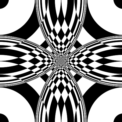
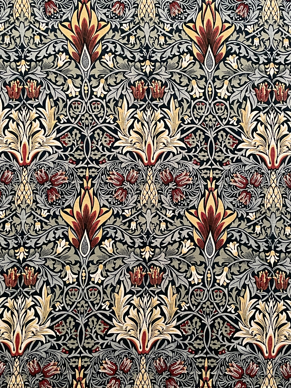
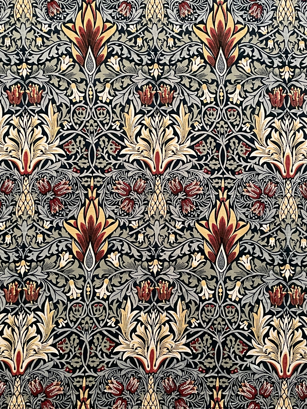
Linear decimation: (a) original image; (b) size = 1 (identity); (b) decimated = 1/3; (c) size = 3, decimated = 1/3; (d) decimated = 1/9; (e) size = 9, decimated = 1/9; (f) decimated = 1/27; (g) size = 27, decimated = 1/27 Linear decimation: (a) original image; (b) size = 1 (identity); (b) decimated = 1/3; (c) size = 3, decimated = 1/3; (d) decimated = 1/9; (e) size = 9, decimated = 1/9; (f) decimated = 1/27; (g) size = 27, decimated = 1/27 Linear decimation: (a) original image; (b) size = 1 (identity); (b) decimated = 1/3; (c) size = 3, decimated = 1/3; (d) decimated = 1/9; (e) size = 9, decimated = 1/9; (f) decimated = 1/27; (g) size = 27, decimated = 1/27 Linear decimation: (a) original image; (b) size = 1 (identity); (b) decimated = 1/3; (c) size = 3, decimated = 1/3; (d) decimated = 1/9; (e) size = 9, decimated = 1/9; (f) decimated = 1/27; (g) size = 27, decimated = 1/27Figures 31{reference-type="ref" reference="fig:linear_decimation_fabric"}, 32{reference-type="ref" reference="fig:linear_decimation_nyc"}, 33{reference-type="ref" reference="fig:linear_decimation_syth1"} and 34{reference-type="ref" reference="fig:linear_decimation_syth2"} show us exactly the difference between an uninterpolated and an interpolated decimation. Especially when it comes to very small photo sizes and synthetic images, the improvement of applying interpolation is impressive. Even for the smallest sizes where the detail is no longer visible, the difference between one image and the other is very noticeable.
def pascal_triangle(n):

    '''
    Return the bionomial coefficients for a given row number in the pascal triangle.

    Args:
        n (int): Row number or also number of coefficients.

    Return:
        A list containing the coefficients.
    '''

    # If n is 1 or smaller, return 1 as if it was 1.
    if n <= 1:
        return [1]

    # Get the coefficients for n-1.
    prev_coeffs = pascal_triangle(n - 1)

    # Get the central part.
    central_part = [prev_coeffs[i - 1] + prev_coeffs[i] for i in range(1, len(prev_coeffs))]

    # Append two ones and return it.
    return [1] + central_part + [1]

def binomial_filter(img, kernel_size):

    '''
    Applies a Binomial filter to all channels.

    Args:
        img (np.array): An RGB image.
        kernel_size (number): Size of the kernel that will be used to compute the convolution.

    Returns:
        The resulting image after applying the convolution.

    See:
        https://research.cs.wisc.edu/graphics/Courses/559-f2002/lectures/cs559-7.ppt
    '''

    # Make sure the kernel size is an odd number. Otherwise, make it odd by adding one and print a
    # warning.
    if kernel_size % 2 == 0:
        kernel_size += 1
        print_debug('Kernel size must be odd. The value used will be {}'.format(kernel_size))

    # Get the bionomial coefficients for this kernel size.
    kernel_gen = np.array([pascal_triangle(kernel_size)])

    # Convert them into two nxn arrays. One vertical and one horizontal.
    kernel = np.dot(np.transpose(kernel_gen), kernel_gen)

    # Convolve all channels using this kernel.
    ret_img = convolve_all_channels(img.astype('uint64'), kernel, True)

    # Normalize the image.
    ret_img = ret_img // np.sum(kernel)

    return ret_img.astype('uint8')
Binomial filtering is a type of convolution in which the kernel is obtained as a multiplication of a binomial coefficient matrix and its transposed matrix.
The code above these lines shows the binomial_filter function that computes the binomial kernel and then convolves the image with it. To get the binomial coefficients needed to perform the matrix multiplication, it uses the pascal_triangle function. The latter obtains the binomial coefficients for a given number of iterations.
fil_img = binomial_filter(org_img, sz)
fil_img = decimate(fil_img, sz)Figures 35{reference-type="ref" reference="fig:binomial_decimation_fabric"}, 36{reference-type="ref" reference="fig:binomial_decimation_nyc"} and 38{reference-type="ref" reference="fig:binomial_decimation_syth2"} show very similar results to those obtained using the Linear interpolation. However, when it comes to Figure 37{reference-type="ref" reference="fig:binomial_decimation_syth1"} a noticeable improvement can be appreciated. This behaviour is due to the shape of the patterns in the image, but a notable improvement has been done in reducing blur when decimating.
The Gaussian decimation uses the Gaussian blur filter that was implemented in previous sections. Therefore, there is no need to discuss its functioning or its implementation again.
Gaussian decimation: (a) original image; (b) size = 1, σ = 0.5 (identity); (b) decimated = 1/3; (c) size = 3, σ = 0.5, decimated = 1/3; (d) decimated = 1/9; (e) size = 9, σ = 0.5, decimated = 1/9; (f) decimated = 1/27; (g) size = 27, σ = 0.5, decimated = 1/27 Gaussian decimation: (a) original image; (b) size = 1, σ = 0.5 (identity); (b) decimated = 1/3; (c) size = 3, σ = 0.5, decimated = 1/3; (d) decimated = 1/9; (e) size = 9, σ = 0.5, decimated = 1/9; (f) decimated = 1/27; (g) size = 27, σ = 0.5, decimated = 1/27 Gaussian decimation: (a) original image; (b) size = 1, σ = 0.5 (identity); (b) decimated = 1/3; (c) size = 3, σ = 0.5, decimated = 1/3; (d) decimated = 1/9; (e) size = 9, σ = 0.5, decimated = 1/9; (f) decimated = 1/27; (g) size = 27, σ = 0.5, decimated = 1/27 Gaussian decimation: (a) original image; (b) size = 1, σ = 0.5 (identity); (b) decimated = 1/3; (c) size = 3, σ = 0.5, decimated = 1/3; (d) decimated = 1/9; (e) size = 9, σ = 0.5, decimated = 1/9; (f) decimated = 1/27; (g) size = 27, σ = 0.5, decimated = 1/27Figures 39{reference-type="ref" reference="fig:gaussian_decimation_fabric"} and 40{reference-type="ref" reference="fig:gaussian_decimation_nyc"} show an improvement when comparing them to the linear interpolation, as they allow more detail to pass through the decimation than before.
However, when it comes to Figures 41{reference-type="ref" reference="fig:gaussian_decimation_syth1"} and 41{reference-type="ref" reference="fig:gaussian_decimation_syth1"} little to no improvement seems to be happening when comparing it to the Binomial decimation.
Gaussian and Binomial seem to be obtaining very similar results when applied to decimation.
As it was stated for the linear decimation, a median filter is essentially a linear interpolation filter. Therefore, to apply linear interpolation to upscaling the same filter can be used by inverting the operations order.
fil_img = upscale(org_img, sz)
fil_img = median_filter(fil_img, sz, sz)Figures 43{reference-type="ref" reference="fig:linear_interpolation_syth1"} and 44{reference-type="ref" reference="fig:linear_interpolation_nyc"} show outstanding results for the linear interpolation upscaling. The images are in line with the original images while showing little artefacts and unexpected shapes.
# Apply the filter and then decimate.
fil_img = upscale(org_img, sz)

channels = split_channels(fil_img)
channels = [bilateral_filter(c, sz, sz, sz/2) for c in channels]
fil_img = merge_channels(channels)
None of the sources consulted for this project discussed bilateral interpolation for image upsampling. However, intuitively could have some attractive results if its ability to smooth flat surfaces while maintaining hard edges during interpolation.
Therefore, this experiment was included in the report to discuss why it got the results it did.
Bilateral interpolation: (a) original image; (b) upscaled = 3/1, size = 3, σr = 3, σs = 1.5; (c) upscaled = 9/1, size = 9, σr = 9, σs = 4.5; (d) upscaled = 27/1, size = 27, σr = 27, σs = 13.5. Bilateral interpolation: (a) original image; (b) upscaled = 3/1, size = 3, σr = 3, σs = 1.5; (c) upscaled = 5/1, size = 5, σr = 5, σs = 2.5; (d) upscaled = 7/1, size = 7, σr = 7, σs = 3.5.fil_img = upscale(org_img, sz)The upscale method in this project actually implements a nearest neighbours method. As its behaviour has already been described in section 7.1, it won't be repeated here.
Bilateral interpolation: (a) original image; (b) upscaled = 3/1; (c) upscaled = 9/1; (d) upscaled = 27/1. Nearest neighbour interpolation: (a) original image; (b) upscaled = 3/1; (c) upscaled = 5/1; (d) upscaled = 7/1.
