Submitted By: Syed Farhan Ahmad
Date of Submission: 9th September, 2020
Time of Submission: 5:30pm IST
- Problem Statement
- Instructions to Run Program
- Ideal Circuit
- Solution Architecture
- Data Encoding
- Parameterized Circuit
- Cost Function
- Mean Squared Error
- Optimizers
- Results and Comparison
- Bonus Question
- Future Scope
Implement a circuit that returns |01> and |10> with equal probability.
Requirements
-
The circuit should consist only of CNOTs, RXs and RYs.
-
Start from all parameters in parametric gates being equal to 0 or randomly chosen.
-
You should find the right set of parameters using gradient descent (you can use more advanced optimization methods if you like).
-
Simulations must be done with sampling - i.e. a limited number of measurements per iteration and noise.
-
Compare the results for different numbers of measurements: 1, 10, 100, 1000.
- Install
qiskit - Execute
python main.py

- The Bell State can be created by the follwing steps:
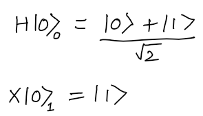
- Applying
H Gateto Qubit 0, andX Gateto qubit 1.
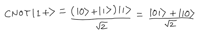
- Applying CNOT gate to the combination


- The problem statement can be solved using a Hybrid Classical-Quantum Optimization approach.
- The Quantum Circuit is implemented using the
BellStateCircuitclass inqpower_app.py. - The Loss function, optimizer function and backpropagation are implemented in
GradientDescentOptimizerclass inqpower_app.py.

- Input data is the parameter
angle_degrees, in degrees, which is the angle by which the paraterized gate will rotate. - The angle is converted to
radiansfromdegrees. - Data is mapped before execution using
parameter_bindsof theqiskit.executefunction inqpower_app.py.
- The parameterized circuit is created using the
qiskit.rygate, that takesangle_degreesas the input parameter. - Qubit 0 is initialized to statevector [1,0], and Qubit 1 to [0,1] to be able to reach the aforementioned Bell State.
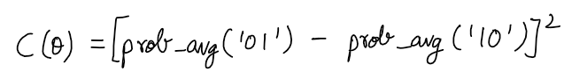
- The Cost function is a simple MSE function that can easily be used with the first order derivative optimizers like Gradient Descent very easily.
- The cost function is the squared difference of the Probability averages of both states
|01>and|10>, that are obtained after the circuit is executed for a given number ofshots.

- The Gradient Descent Optimizer is being used as it simplifies the process of loss convergence when our loss function is quadratic in nature.
- The local and global minima are the same and the
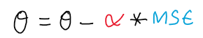
loss landscapecan be easily analysed with much less compute power, and good accuracy. - The parameter
angle_degreesis being learned, using Gradient Descent and alpha is thelearning_rate.

- Coming soon

- The results are taken for all measurements 1, 10, 100 and 1000 respectively.
- The error of measurement is less than 1.5% in all cases as seen.
- Expected output: 90 degrees(or a multiple of 90 degrees)
How to make sure you produce state |01> + |10> and not |01> - |10> ?
- To prevent the occurrence of the state
|01> - |10>, we will have to alter our cost function to be unsymmetrical. To alter the Mean Sqared error, we can remove the squares and keep the function linear. - This can be done by the following:
prob_avg_10 - (prob_avg_01+prob_avg_10)/(2)
- Use of better Optimizer functions like
NAG(Nesterov Accelerated Gradient) Hessianbased analysis of the Loss Landscapes- etc.