Manipulate in Python

Description

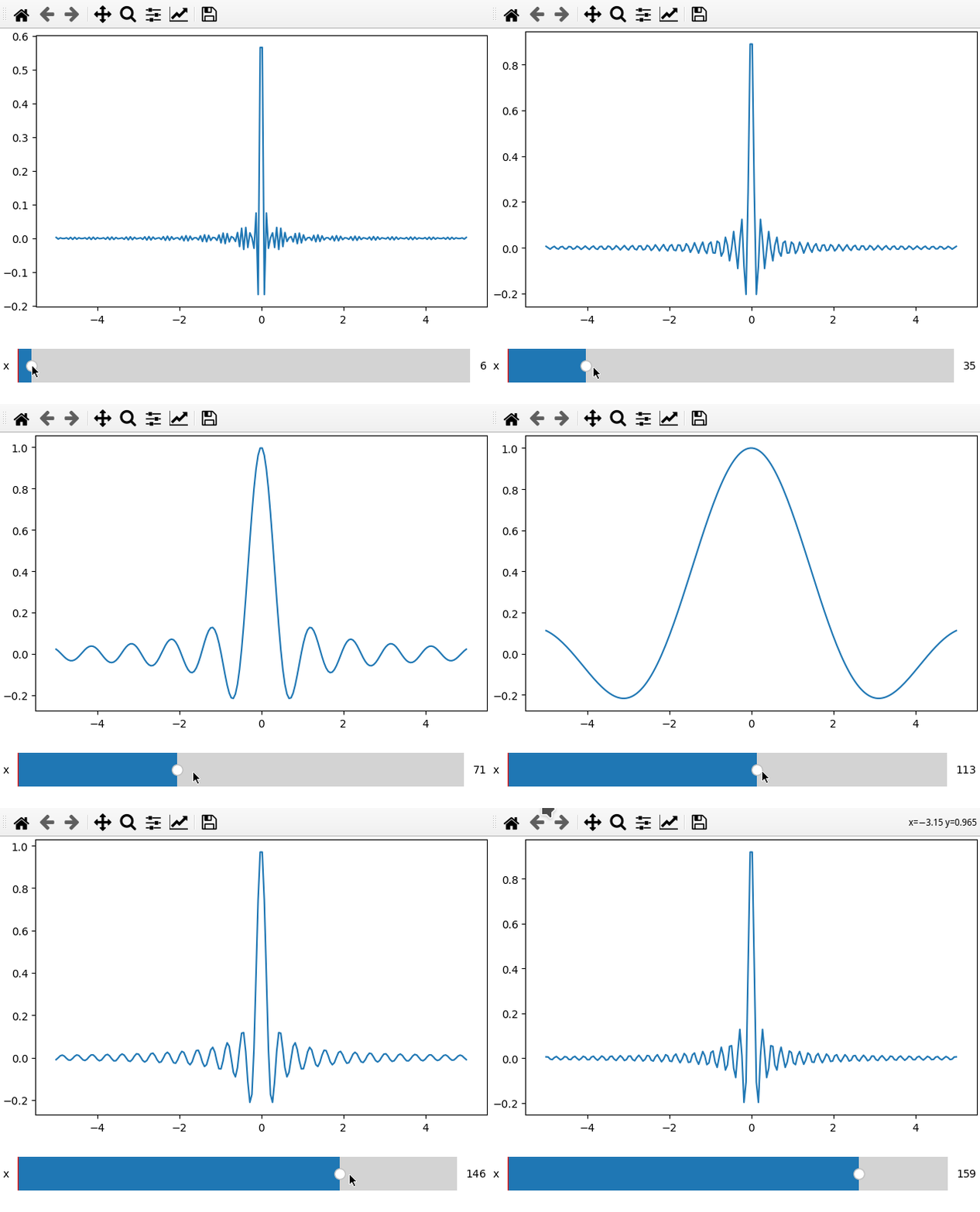
The package repository is located at https://github.com/bottom-bracket/manipylate. It can also be installed from pypi with pip install manipylate.

In research we spend some time with plotting data, comparing measurement results or testing the influence of parameter changes. Often the most intuitive approach is by looking at different plots. However, while python is great to create reproducible figures, I found no way to quickly create plots with which one can interact without changing the code used to create the plot as in mathematica’s Manipulate. The closest one can get to this is interact from ipywidgets which is limited to run in Jupyter notebooks.

Manipylate shall provide the simplified functionalities from its bigger sibling Manipulate. The tasks I had in mind while writing the tool are:

Plotting 1d and 2d cuts of multidimensional data and changing the slice index with sliders
Plot a function for changing parameters which one can modify interactively

I also wanted to keep things as simple as possible and be able to use manipylate outside jupyter notebooks.

Interactivity

Sliders are added automatically
Views can be saved with Shift + middle mouse click in the figure if used in pure matplotlib mode and by click on the camera button in jupyter

Examples

First we get the environment ready (leave out the lines starting with % for non-ipython shells).

%matplotlib qt
%load_ext autoreload
%autoreload 2
import matplotlib as mpl
from matplotlib import pyplot as plt
import numpy as np
from manipylate import ifigure

1d cut through a 2d array

Let’s create some data:

x = np.linspace(-5, 5, 200)
X, Y = np.meshgrid(x, x)
data = np.sinc(X * Y**2)

The figure is created by creating an ifigure object. We can then call its add_plot method to add an axis and a line plot. Here axpos defines where the plot shall be placed, x is the x-axis data. data the 2d array of which we want to plot a cut along the axis given by plot_ax, and parameters is a list of dimension parameters we want to change using sliders.

Calling show creates the figure. It needs to be called after all plots have been added to the figure since here we’ll create the sliders and arange the slider axes (in case of execution outside jupyter).

ifig = ifigure(1,1)
ifig.add_plot(axpos=[0,0],x=x,data=data,parameters=['x'],plot_ax=1)
ifig.show()

In jupyter notebook

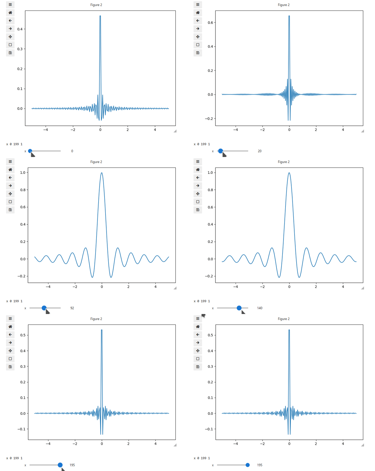
In order to use the ipywidget widgets, we call ifigure with the jupyterwidget keyword argument.

ifig = ifigure(1,1,jupyterwidget=True)
ifig.add_plot(axpos=[0,0],x=x,data=data,parameters=['x'],plot_ax=1)
ifig.show()

Adding a second plot

In the same axis

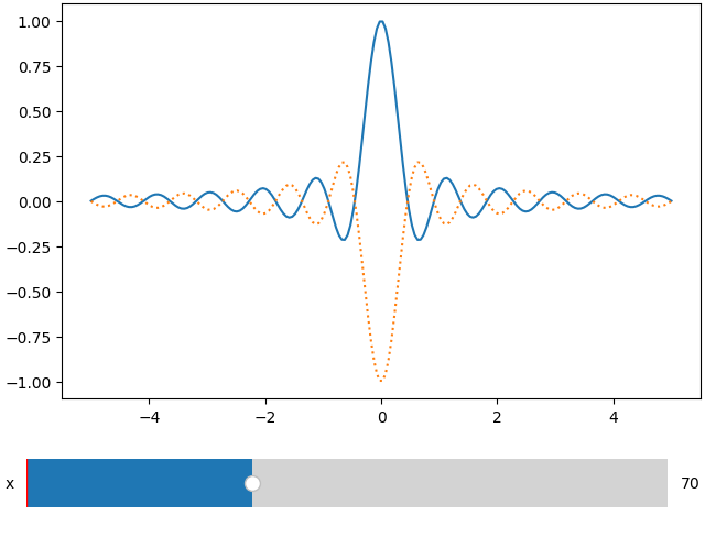
Axes are remembered by the ifigure object based on their position, so we can call the same add_plot command with another dataset. Note that any keyword arguments are passed to matplotlib.axes.plot, so we can use this to change the line style.

ifig = ifigure(1,1)
ifig.add_plot(axpos=[0,0],x=x,data=data,parameters=['x'],plot_ax=1)
ifig.add_plot(axpos=[0,0],x=x,data=-data,parameters=['x'],plot_ax=1,ls=':')
ifig.show()

Note that here both plots share the same parameter. In the next example we will see that if called with a different name, a new slider will be created.

As twinned axis

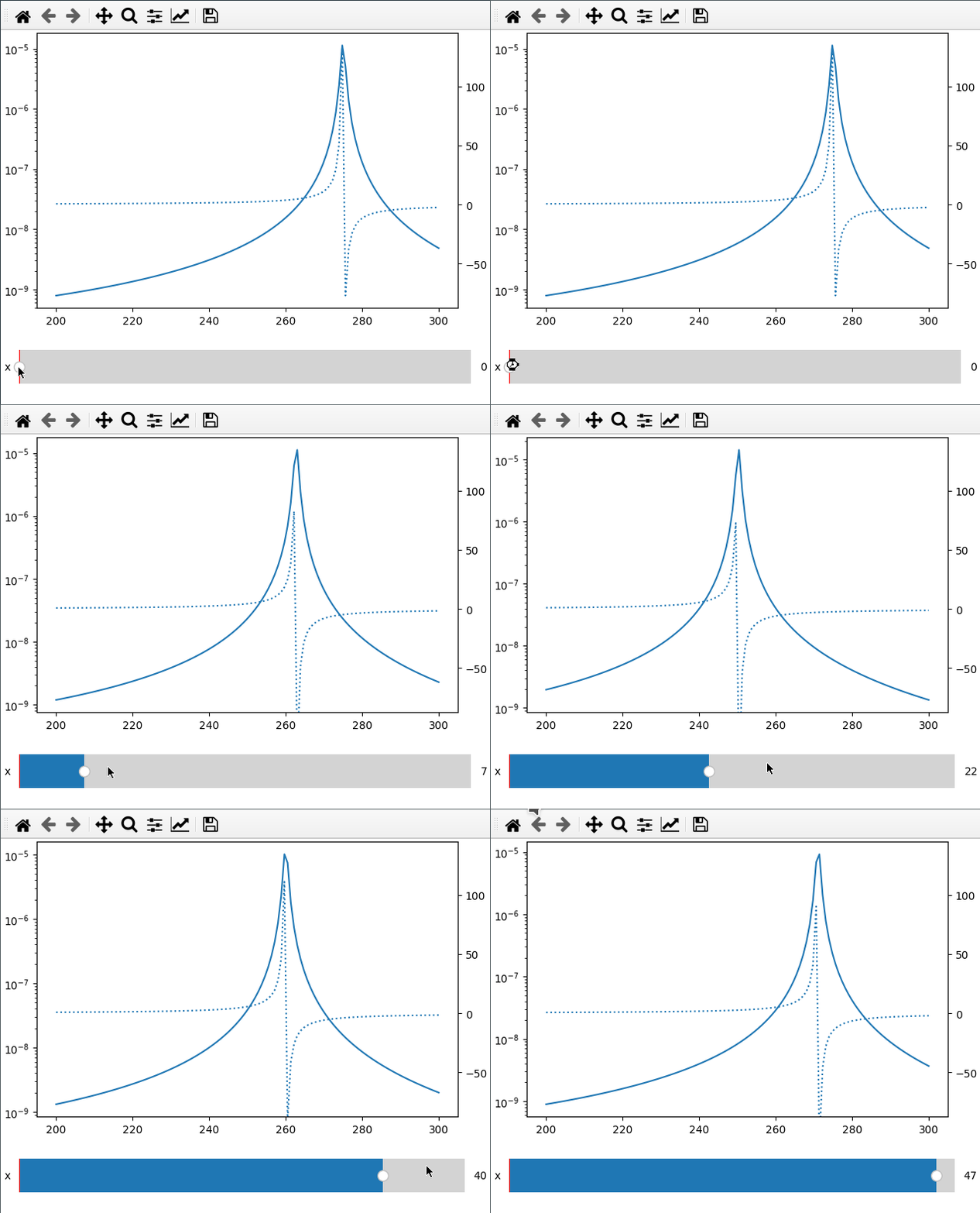
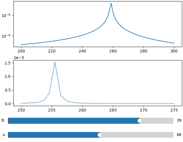
Sometimes I want to compare two different values (like amplitude and phase) over the same x axis. This can be done by passing the twinx=True to the add_plot method. Here I also use the fix_lim flag to prevent the phase axis from updating. Note that add_plot returns a matplotlib axis instance which we can modify as usual (here setting the y scale to logarithmic).

fc = np.linspace(-5, 5, 50) ** 2 + 250
x = np.linspace(200, 300, 120)
FC, X = np.meshgrid(fc, x, indexing="ij")
data = 1 / ((FC ** 2 - X ** 2 - 1j * X * 1) ** 2)

ifig = ifigure(1, 1)
ax = ifig.add_plot(axpos=[0, 0], x=x, data=np.abs(data), parameters=["fc"], plot_ax=1)
ax.set_yscale("log")
ifig.add_plot(
    axpos=[0, 0],
    x=x,
    data=np.angle(data, deg=True),
    parameters=["x"],
    plot_ax=1,
    twinx=True,
    ls=":",
    fix_lim=True,
)
ifig.show()

As new axis

In order to add more than one subplots we adjust the ifigure creation. Here we also use another parameter for the second plot.

fc = np.linspace(-5, 5, 50) ** 2 + 250
x = np.linspace(200, 300, 120)
FC, X = np.meshgrid(fc, x, indexing="ij")
data = 1 / ((FC ** 2 - X ** 2 - 1j * X * 1) ** 2)

ifig = ifigure(2, 1)
ax = ifig.add_plot(axpos=[0, 0], x=x, data=np.abs(data), parameters=["fc"], plot_ax=1)
ax.set_yscale("log")
ifig.add_plot(
    axpos=[1, 0],
    x=fc,
    data=np.abs(data),
    parameters=["x"],
    plot_ax=0,
    ls=":",
)
ifig.show()

2d cut trough nd array

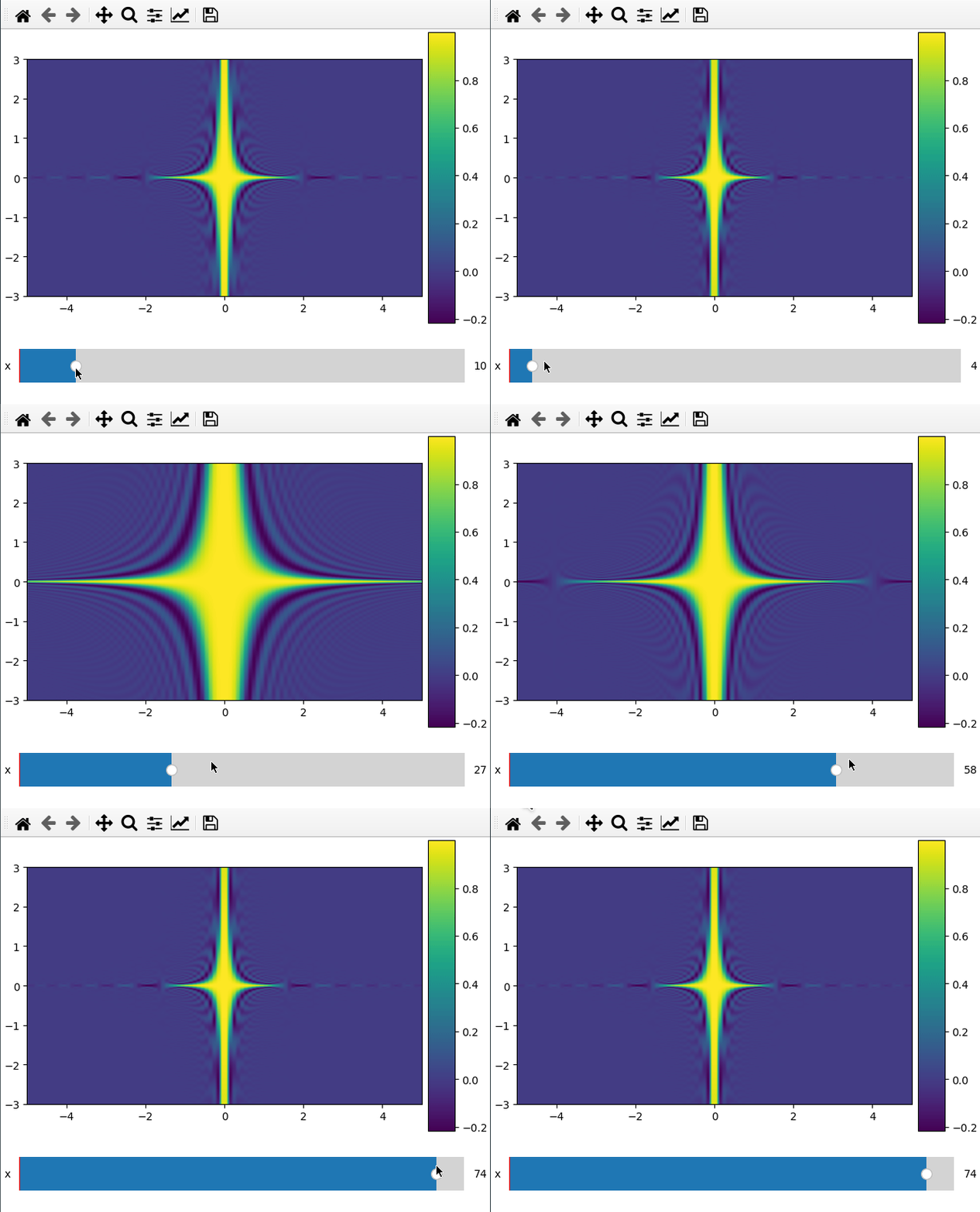
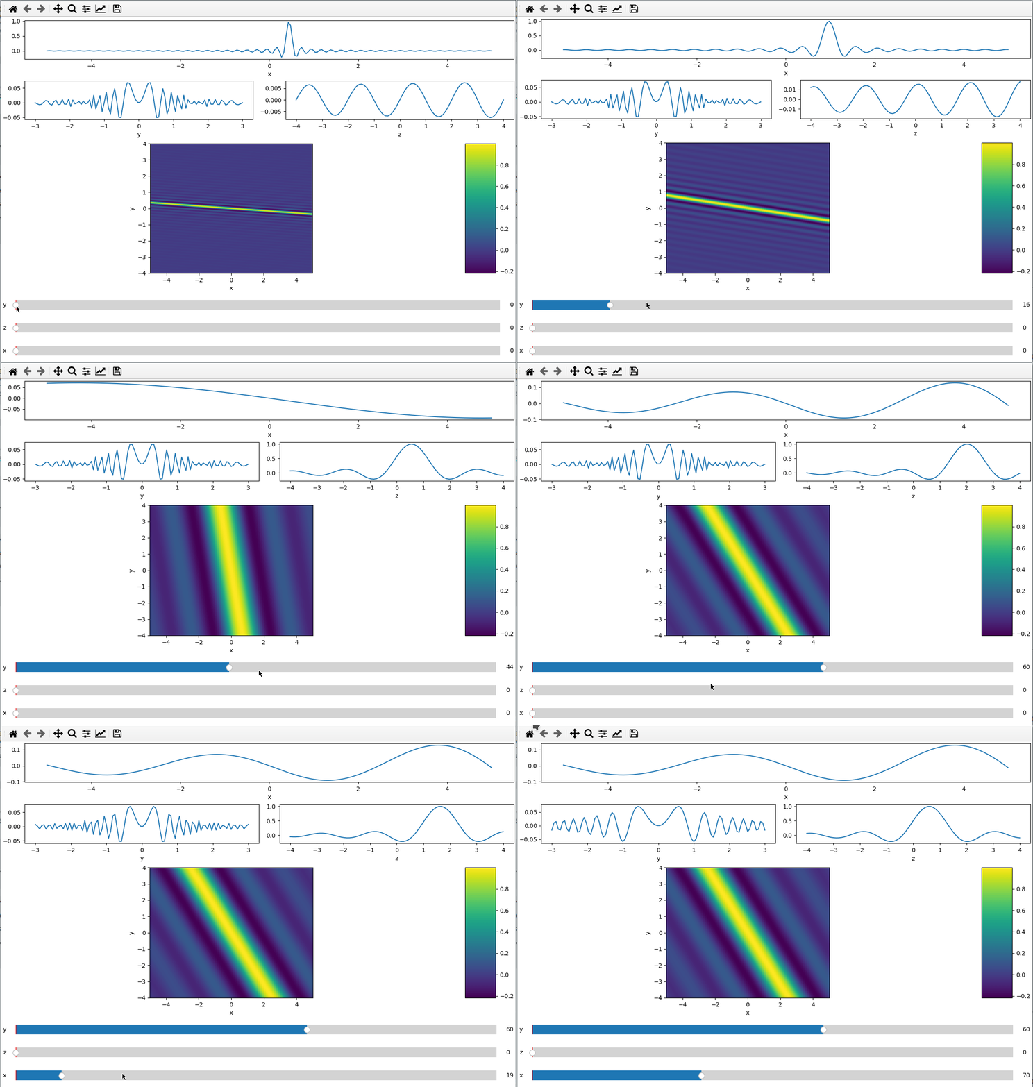
Plotting a 2d cut is nearly the same as a 1d line. ifigure creates an imshow plot when being passed data which has two more dimensions than the number of parameters passed to the function. For the 2d plot we need to specify along which axes we want to cut by changing the plot_ax argument to a list of length 2.

x = np.linspace(-5, 5, 200)
y = np.linspace(-3, 3, 100)
z = np.linspace(-4, 4, 80)
X, Y ,Z = np.meshgrid(x, y, z,indexing='ij')
data = np.sinc(X * Y**2 * Z**3)

ifig=ifigure(1,1)

ifig.add_plot(axpos=[0,0],x=[x,y],data=data,parameters=['x'],plot_ax=[0,1])
ifig.show()

Plotting a functions value

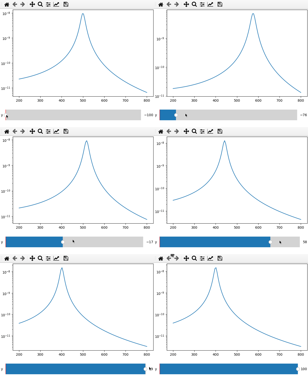
The data argument can be replaced by a function that returns either a 1d array for a line plot or a 2d array for a map plot.

In 1d

The main difference to calling the plot on an array is that we do not need to specify the plot_ax parameter but we need to define a range and step size for the slider, which is done by replacing the string argument in the parameter list by a list containing name,minimum, maximum and step size.

fc = 250
x = np.linspace(200, 800, 120)
def lor(y):
    return np.abs(1 / ((4*fc ** 2 - (x+y) ** 2 - 1j * x * 20) ** 2))

ifig = ifigure(1, 1)
ax = ifig.add_plot(axpos=[0, 0], x=x, data=lor, parameters=[["y",-100,100,1]])
ax.set_yscale("log")
ifig.show()

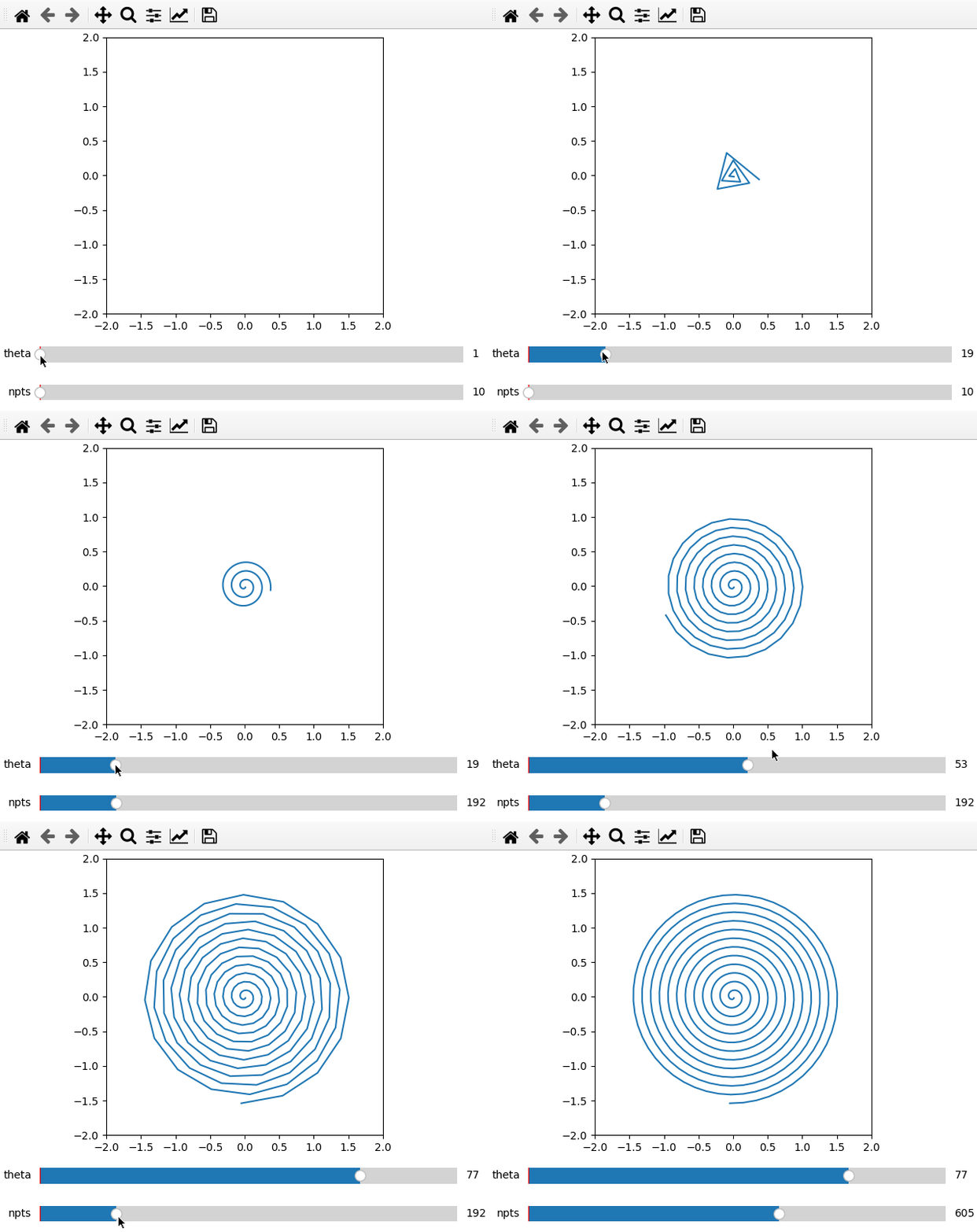
Furthermore it is possible to do parametric plots using a function for x and data arguments. Make sure that the variable names are the same in the definition and add_plot call.

import numpy as np
from manipylate import ifigure

def x(theta,npts):
    th = np.linspace(1,theta,npts)
    return th/50*np.cos(th)
def y(theta,npts):
    th = np.linspace(1,theta,npts)
    return -th/50*np.sin(th)

ifig = ifigure(1,1)
ax = ifig.add_plot(axpos=[0,0],x=x,data=y,parameters=[['theta',1,100,1],['npts',10,1000,1]],fix_lim=True)
ax.set_ylim(-2,2)
ax.set_xlim(-2,2)
ax.set_aspect('equal')
ifig.show()

If one of the functions x,y takes more arguments than the other just add a **kwargs to its definition (e.g. def x(theta,npts,**kwargs)).

In 2d

Complex figure layout

Since the subplot layout creation is based on GridSpec, we can create more complicated layouts. We use the handy numpy.s_ to create the exact slices to index the GridSpec.

x = np.linspace(-5, 5, 200)
y = np.linspace(-3, 3, 100)
z = np.linspace(-4, 4, 80)
X, Y ,Z = np.meshgrid(x, y, z,indexing='ij')
data = np.sinc(X * Y**2 + Z)

ifig = ifigure(6, 4,figsize=(12,8))
ax=ifig.add_plot(axpos=np.s_[0,:], x=x, data=data, parameters=["y",'z'],plot_ax=0)
ax.set(xlabel='x')
ax=ifig.add_plot(axpos=np.s_[1,:2], x=y, data=data, parameters=["x","z"],plot_ax=1)
ax.set(xlabel='y')
ax=ifig.add_plot(axpos=np.s_[1,2:], x=z, data=data, parameters=["x","y"],plot_ax=2)
ax.set(xlabel='z')
ax=ifig.add_plot(axpos=np.s_[2::,:], x=[x,z], data=data, parameters=["y"],plot_ax=[0,2])
ax.set(xlabel='x',ylabel='y')
ifig.show()

Naming and saving views

The ifigure class can be called with the figurename parameter which will determine the base name and the extension for individually saved views. The full filename is constructed from the figurename and the current slider names and values. Slider axes are removed during saving.

TODOs

Comment and document code

Bugs

Missing Features

add convert_param method to display physical parameter values (e.g. 0-1μm instead of index values 1-51)
3d plots ?
choice for 2d plots (contour)