The goal of scDNA R package is to provide a simple framework for analyzing single cell DNA sequencing data. The current version primarily focuses processing variant information on the Mission Bio Tapestri platform. Functionality includes import of h5 files from Tapestri pipeline, basic variant annotation, genotype extraction, clone identification, and clonal trajectory inference. This package provides wrappers for normalizing protein data for scDNA+Protein libraries for downstream analysis.
You can install (re-install) the current version (1.1) of scDNA below
remotes::install_github("bowmanr/scDNA",force=TRUE)Version 1.1 is finally here with exciting new developments:
- New sequencing panels for variant annotation introduced:
- hg38
- mm10
- New plotting functions for RL trajectories.
- new interactive plots,
- BSCITE-style implementation.
- Demultiplexing samples is introduced
- (integrated and adapted from Robinson et al, github)
- vignette included to demonstrate how to perform it.
- Cell confidence labeling based on DNA and Protein data.
- Outlier scores introduced for cell confidence.
- Stain index introduced for cell confidence.
- Copy number variation (CNV) and Ploidy analysis introduced.
- Allele dropout assessment introduced.
-
H5 files are now read using the rhdf5 package and stored into a SingleCellExperiment container.
-
Merged h5 samples are identified and sample names are stored in colData(). Variant identification is ran separately and then merged.
-
Variant information is stored in rowData()
-
NGT matrix, clonal abundance, and clone architecture familiar to previous versions can be found in the metadata.
-
-
Variant identification and annotation is performed initially before reading in all the genotyping/QC data.
-
Transcript annotation matches cannonical transcripts used in the cBio portal.
-
To decrease variant location identification runtime, we created a custom TxDB object for the Clonal Evolution Panel from used here. If you have a different panel you can also use the TxDB for hg19 from UCSC. Future versions will have local data for all panels from Mission Bio, as well as a simple script for generating a TxDB object for custom panels.
-
-
Protein data is stored as an altExp() container within the container.
Identify all variants within a sample.
library(scDNA)
library(dplyr)
sample_file<- "test_file.h5"
variant_output<-variant_ID(file=sample_file,
                           panel="MSK_RL", # "UCSC" can be used for other panels
                           GT_cutoff=0,  # mimimum percent of cells where a successful genotyping call was made
                           VAF_cutoff=0) # mimimum variant allele frequency
Identify mutations in genes of interest.
genes_of_interest <- c("IDH2","NRAS","NPM1","TET2","FLT3","IDH1")
variants_of_interest<-variant_output%>%
                          dplyr::filter(Class=="Exon")%>%
                          dplyr::filter(VAF>0.01)%>%
                          dplyr::filter(genotyping_rate>85)%>%
                          dplyr::filter(!is.na(CONSEQUENCE)&CONSEQUENCE!="synonymous")%>%
                          dplyr::filter(SYMBOL%in%genes_of_interest)%>%
                          dplyr::arrange(desc(VAF))%>%
                          dplyr::slice(c(1:3)) # take the 3 most abundance mutations
Read in the data, enumerate clones, and compute statistics. Sample statistics mirror that seen in Figure 1 here, and are stored in the metadata.
sce<-tapestri_h5_to_sce(file=sample_file,variant_set = variants_of_interest)
sce<-enumerate_clones(sce)
sce<-compute_clone_statistics(sce,skip_ploidy=FALSE)
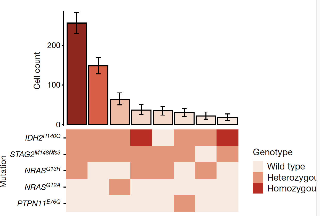
Simple function for producing a graph in the style of Figure 1D from here,
clonograph(sce)Function to perform Reinforcment Learning / MDP approach for clonal trajectory as in Figure 3 here,
sce<-trajectory_analysis(sce,use_ADO=TRUE)Methods for protein normalization. Both dsb and CLR normalization can be performed and stored in separate slots. We tend to have favor dsb so far.
droplet_metadata<- extract_droplet_size(sce)
background_droplets<-droplet_metadata%>%
                          dplyr::filter(Droplet_type=="Empty")%>%
                          dplyr::filter(dna_size<1.5&dna_size>0.15)%>%
                          pull(Cell)

sce<-normalize_protein_data(sce=sce,
                             metadata=droplet_metadata,
                             method=c("dsb","CLR"),
                             detect_IgG=TRUE,
background_droplets=background_droplets)- Cohort summarization
- Creating custom TxDB objects
- Improving cell identification and distinction from empty droplets.
- Doublet and dead cell identification
- Improve normalization for protein data.
- Improve cell type identification based on immunophenotype
- Improvements to the MDP and RL.
