PSY-P457 Code, data, and examples

This repository contains data, code, and assignments for students enrolled in PSY-P457: Networks in the psychological, cognitive, and brain sciences.

To make your lives easier, I have included a few examples where I illustrate how to perform some basic operations.

How do I load connectivity data?

Datasets that we need for the course are in the data/ directory and, unless noted otherwise, stored as .mat files. This file type is specific to MATLAB--you can think of .mat files as bags or boxes in which many variables, including connectivity data, can be stored. When we load a .mat file, we are loading many variables into our workspace.

By default, the datasets included in data/ come from the Brain Connectivity Toolbox. Once you've cloned or downloaded this repository, you can create all of your scripts in the m directory. Right now, that directory is empty. If we wanted to load data from a script located in m, we'd write something like:

% load a .mat file from a specific location
load('../mat/Coactivation_matrix.mat')

Note here that the ../mat/ tells MATLAB to go navigate to one directory higher than m and then into the mat directory. It then specifies the exact file to load. In this case, it's one named Coactivation_matrix.mat. If you replaced Coactivation_matrix.mat with mac95.mat then you'd load a different .mat file.

It is also critical that you specify the correct path to the file you're trying to load. For instance, if you wrote:

% load a .mat file from a specific location
load('../directory_x/Coactivation_matrix.mat')

and directory_x doesn't exist, then the above command would return an error.

How do I call a function or load data from a different directory?

MATLAB can only ``see'' the files located in your current directory You can figure out your current directory by looking in the "Path bar" at the top of the MATLAB GUI, the "Current Folder" tab, or by typing either of the following commands in the "Command Window":

% display current directory (doesn't assign to a variable)
cd

% assign current directory to a variable name
working_directory = pwd;
disp(working_directory);

If you want to be able to access from directory X a file saved in directory Y, then you need to execute the following.

% navigate to directory Y and execute
path_to_y = pwd;

Once you've done this, return to directory X and write:

addpath(path_to_y);

Now you can run functions or load files located in directory Y while your current folder is directory X.

How do I calculate the number of nodes and connections in my network?

Suppose you've already loaded some data using syntax borrowed from the previous section. Let's also suppose that the variable Cij denotes your connectivity matrix. If we wanted to calculate the number of nodes and connections in the network (irrespective of their weights), we could write the following:

% calculate number of nodes
n_nodes = length(Cij);

% calculate the number of nonzero entries in the matrix
n_edges = nnz(Cij);

% calculate the density of connections (fraction of existing edges divided by total number possible)
dens = density_und(Cij); % <- if your network is undirected
dens = density_dir(Cij); % <- if your network is directed

How do I calculate the number of connections each node makes?

The number of connections a node makes is referred to as its degree. For directed networks, we can further break down this number by parsing degree into the number of incoming and outgoing connections. If we wanted to calculate nodes' degrees, we could use the following functions:

% calculate incoming/outgoing/total degree for each node in a directed network
[degree_in,degree_out,degree_tot] = degrees_dir(Cij);

% do the same for nodes in an undirected network
degrees = degrees_und(Cij);

How do I calculate global measures like characteristic path length and efficiency?

The simplest way to do this for any network is to calculate the shortest paths matrix between all pairs of nodes. Again, supposing our connectivity matrix is Cij, we would write the following:

% calculate distance matrix
D = distance_bin(Cij);

% calculate binary path length and efficiency
[lambda,efficiency] = charpath(D);

In the above lines, lambda and efficiency are the path length and efficiency of the network.

The above procedure works for a binary network where edges are either 1 or 0. For weighted networks, we can do something similar, but have to first convert our edge weights from measures of affinity (how much two nodes ``like'' one another) to how costly each edge is. We can do that like so:

% transform weights into costs via an inversion
Cost = 1./Cij;

% calculate weighted distance matrix
D_wei = distance_wei(Cost);

% calculate weighted path length and efficiency
[lambda_wei,efficiency_wei] = charpath(D);

How do I get modules and communities?

There are many algorithms for calculating communities -- the simplest is modularity maximization. It is implemented in the Brain Connectivity Toolbox as the community_louvain function. Unlike other measures, it is not deterministic and is instead stochastic. This means that each time you run the algorithm, you might obtain a different result. So we need to develop a way to address this issue, but let's start with the case where we only want to run the algorithm once.

% run modularity maximization for a network where all edge weights are positive
[Ci,Q] = community_louvain(Cij);

The above lines of code yields two outputs: Ci, which is a vector of community labels for a each node, and Q, which is a measure of the community quality -- i.e. how good the communities are.

As I noted earlier, the community_louvain function is stochastic (you can convince yourself of this by running the algorithm twice and then manually comparing the cluster labels against one another). Ideally, what we want to do is run the algorithm many times and somehow average the slightly dissimilar results together to obtain a set of consensus clusters. This is more involved, but you can do it using the consensus_und function:

% number of times to repeat community detection algorithm
num_iter = 100;

% number of nodes
n_nodes = length(Cij);

% empty array for storing the community labels
Ci = zeros(n_nodes,num_iter);

% run the community detection algorithm num_iter times
for iter = 1:num_iter
  Ci(:,iter) = community_louvain(Cij);
end

% calculate the module coassignment matrix -- for every pair of nodes
% how many times were they assigned to the same community
Coassignment = agreement(Ci)/num_iter;

% node we use the consensus clustering function
thr = 0.5;
cicon = consensus_und(Coassignment,thr,num_iter);

The consensus clustering function is useful--it discards weights below a value of thr and then directly clusters the module coassignment matrix Coassignment. Because the modules are almost always better defined in this matrix than in Cij, they will be easier to detect and the algorithm tends to converge to a partition that emphasizes co-assignments that are consistently observed in the initial set of detected partitions, Ci.

How do I visualize my network data?

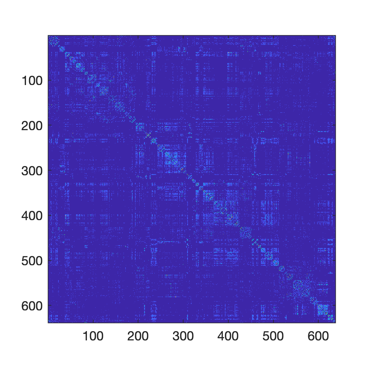
There are a few strategies for visualizing network data. For instance, we can visualize the connectivity matrix using the imagesc command. This command shows the connectivity matrix as a ``grid'' -- the strongest connections are assigned warm colors while non-existent or weak connections are assigned cooler colors. Again, supposing our connectivity data is defined by Cij. In fact, let's make this concrete and use the coactivation matrix from before:

% load the macaque dataset
load('../mat/Coactivation_matrix.mat');

% here, the connectivity matrix is named "Coactivation_matrix", so for the same of continuity, let's just rename it as Cij
Cij = Coactivation_matrix;

% create a figure and use imagesc to visualize the matrix
f = figure;
imagesc(Cij);

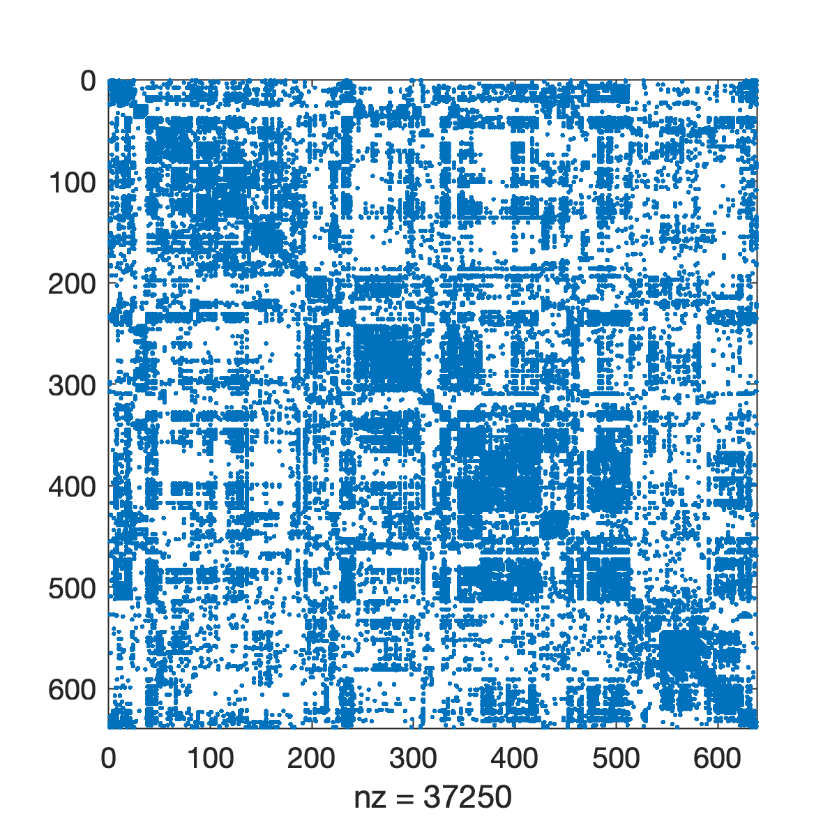
If our network is binary and sparse (only a small fraction of possible connections exist), we can also use the spy command to just highlight connections that exist versus those that do not.

% create a figure and use spy to visualize the matrix
f = figure;
spy(Cij);

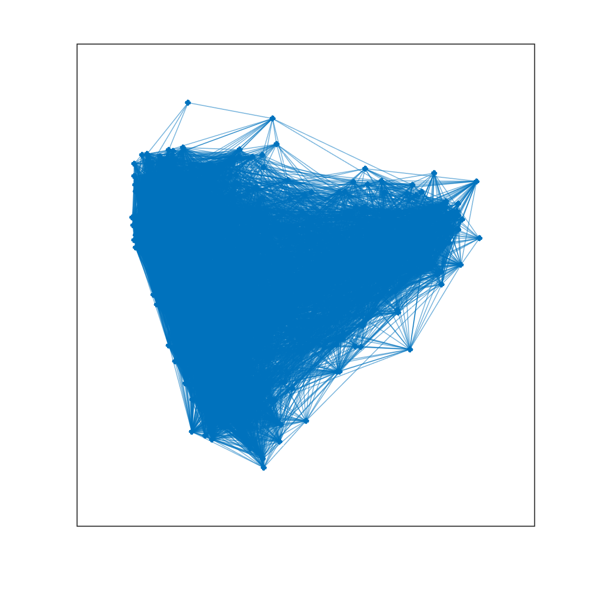
Matlab also gives us the ability to use ``force-directed'' layouts for visualizing our network. The algorithms for generating these layouts imagine that edges are springs and they choose 2D coordinates for each node so as to minimize the spring potential energy of the system.

% create a graph object
g = graph(Cij);

% create a figure and use plot to visualize the network
f = figure;
plot(g);

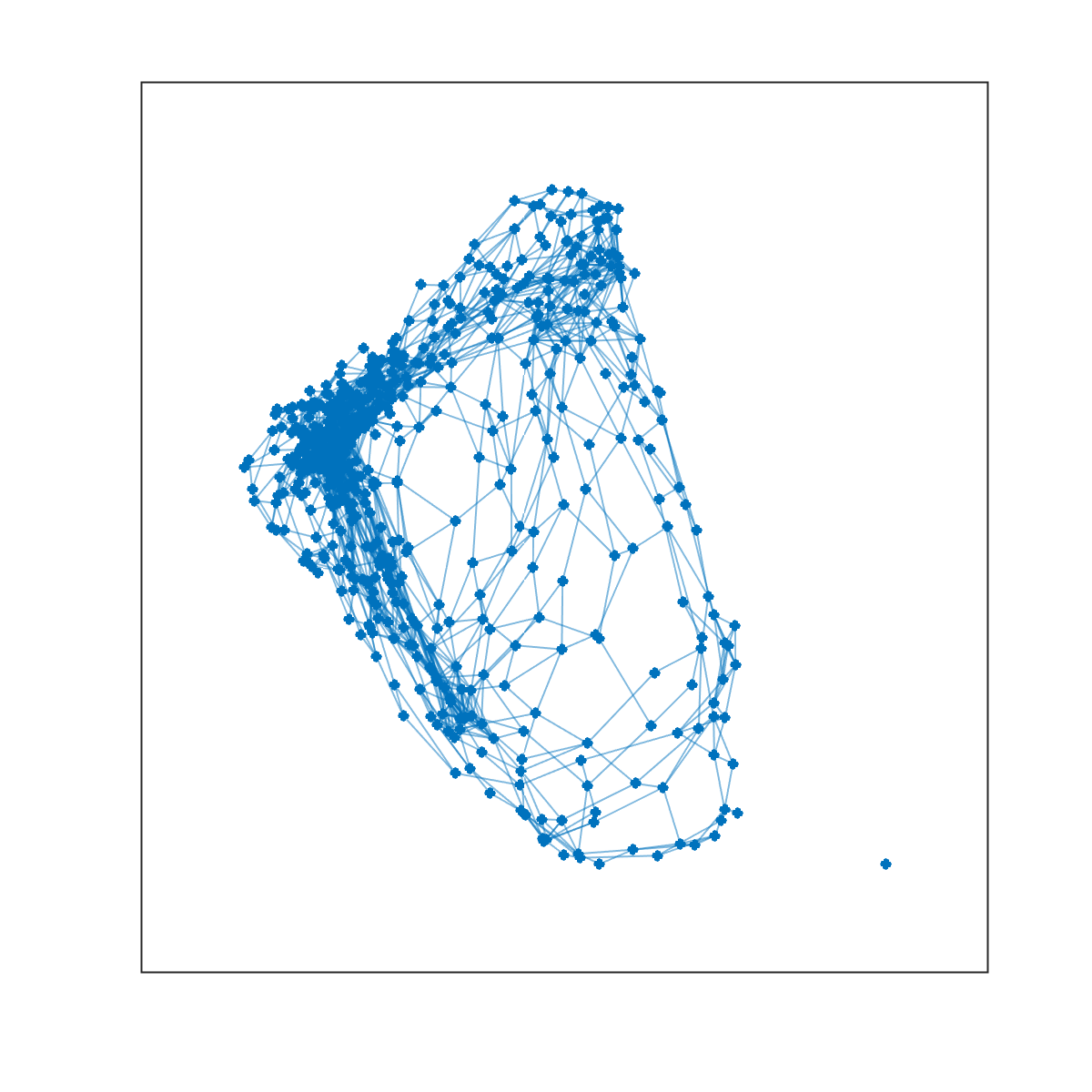
Note that the above figure is very dense and difficult to make much sense of. This is because there are many connections displayed simultaneously, many of which are weak. We can threshold the network and repeat this process, hopefully generating a clearer image.

% threshold the network so that it has 1% connection density
Cij_thresh = threshold_proportional(Cij,0.01);

% create a graph object
g = graph(Cij_thresh);

% create a figure and use plot to visualize the network
f = figure;
plot(g);

I need to generate a "randomized" network. How do I do that?

A lot of times, we measure properties of our observed network. To contextualize those measurements, we need to compare them against a "null distribution." That is, we need to generate randomized versions of our network that preserve key features--e.g. number of nodes, number of connections, each nodes' degree--but where connections are otherwise formed at random.

The Brain Connectivity Toolbox includes several functions for doing this. They have names like randmio_*, where * is either und for undirected networks or dir for networks with directed edges. Let's suppose we're working with the Coactivation_matrix again, which is an undirected network.

This particular class of randomization functions use the Maslov-Sneppen edge-swapping algorithm to generate networks with identical degree sequences as the original network (where each node makes exactly the same number of connections) but where the connections have, otherwise, been randomized.

To generate a randomized surrogate, we write something like this:

% generate a random network where each edge is randomized approximate numiter times
numiter = 32;
Cij_rand = randmio_und(Cij,numiter);

You can visualize the network using any of the above methods to confirm that it looks different than the original network. You can also confirm that its degree sequence is identical plot plotting each node's degree against its degree in the original network.

How do I know if my network is a ``small world''?

Small-world networks have short path length (comparable to a random graph) and large clustering coefficient (comparable to a regular graph). But how do we formally test for this? One strategy is to calculate the ``small-world index'', denoted by the variable $\sigma$. Rather than simply calculating path length and clustering, $L$ and $C$, respectively, we also calculate those same values for an ensemble of random networks, estimating their mean values, $L_r$ and $C_r$ across that ensemble. We the express the original values relative to that of the random networks as normalized coefficients: $L_n = L/L_r$ and $C_n = C/C_r$. We then calculate $\sigma$ as $\sigma = C_n/L_n$.

Intuitively, $L_n \approx 1$ and $C_n >> 1$ for a small world network. Therefore, if $\sigma >> 1$, then we have some evidence that our network is a small-world. The snippet of code below implements this for a binary, undirected network whose adjacency matrix is given by CIJ:

% calculate nodal clustering coefficient
c_node = clustering_coef_bu(CIJ);

% calculate global (mean) clustering
c_global = mean(c_node);

% get distance matrix
spl_bin = distance_bin(CIJ);

% get characteristic path length
l = charpath(spl_bin);

% get number of edges
m = nnz(triu(CIJ,1));

% get number of nodes
n = size(CIJ,1);

% get number of possible edges
k = n*(n - 1)/2;

% get indices for edges
edge_indices = find(triu(ones(n),1));

% number of random networks
nrand = 1000;

% preallocate memory for measures
c_global_random_vec = zeros(nrand,1);
l_random_vec = zeros(nrand,1);

% generate networks
for irand = 1:nrand

    % make a random network
    CIJ_random = zeros(n);
    CIJ_random(edge_indices(randperm(k,m))) = 1;
    CIJ_random = CIJ_random + CIJ_random';

    % calculate global clustering
    c_global_random_vec(irand) = mean(clustering_coef_bu(CIJ_random));

    % calculate characteristic path length
    l_random_vec(irand) = charpath(distance_bin(CIJ_random));

end

% get mean values
c_global_random = mean(c_global_random_vec);
l_random = mean(l_random_vec);

% calculate normalized measures
c_n = c_global/c_global_random;
l_n = l/l_random;

% calculate small-world index
sigma = c_n/l_n;

How do I identify rich-club structure in my data?

Rich-clubs are sub-networks composed of high degree nodes (hubs) that are more densely connected to one another than expected by chance. To detect rich club structure, we identify nodes whose degrees are greater than $k$, and calculate the density of connections between them. This density is denoted as $\phi(k)$ and is referred to as the ``rich-club coefficient''.

It's straightforward to measure this for a real-world network. The time-consuming part is that we need to perform a statistical evaluation of $\phi(k)$. That is, we need to compare its value with a null distribution to determine if our observed rich-club coefficient is greater than expected. To do this, we need to calculate the rich-club coefficient for an ensemble of randomized networks. How do we do this?

% binarize network
CIJ = +(CIJ ~= 0);

% target degree
k = 40;

% calculate nodes' degrees
degrees = degrees_und(CIJ);

% get sub-network
idx = degrees > k;
CIJsub = CIJ(idx,idx);

% get density
phi = density_und(CIJsub);

% generate randomized networks
nrand = 100; % number of randomized networks
nswaps = 32; % number of times each edge is "rewired" on average
for irand = 1:nrand
  CIJrand = randmio_und(CIJ,nswaps);
  CIJrandsub = CIJrand(idx,idx);
  phirand(irand) = density_und(CIJrandsub);
end

% calculate p-value
p = mean(phirand >= phi);

% calculate normalized coefficient
phinorm = mean(phi./phirand);

If the variable p is less than 0.05 (or another statistical criterion) then we can conclude that there's a statistically significant rich-club. Oftentimes, people report a normalized rich-club coefficient as the ratio of the observed coefficient with that of the randomized networks.

When I'm ready to turn in my assignment, what should I give you?

The preferred procedure is as follows. Open your script in MATLAB, click on the Publish tab at the top of the screen. Then press the Publish button (a green ``play'' arrow on top of what looks like an envelop). This will convert your script into an html file. Within the file, it will embed images, code, and comments that were generated as part of your script. Compress/zip those files together and submit them on Canvas. Note: Always check to make sure that the published file contains all the outputs I need to evaluate your submission. For instance, not just the images/figures, but also comments and numerical output.

However, if you have any issue with the publication procedure, you're always welcome to submit the .m file directly. It's a riskier, because then I have to run the code on my own computer and might be missing dependencies, files you load might not be in the same place on my computer as they are on yours, and (in general) more likely to result in errors.

But either option is totally fine!

brain-networks/PSY-P457