A multi-sensor benchmark dataset for detecting individual trees in airborne RGB, Hyperspectral and LIDAR point clouds

Individual tree detection is a central task in forestry and ecology. Few papers analyze proposed methods across a wide geographic area. The NeonTreeEvaluation dataset is a set of bounding boxes drawn on RGB imagery for 22 sites in the National Ecological Observation Network (NEON). Each site covers a different forest type(e.g. TEAK). This dataset is the first to have consistant annotations across a variety of ecosystems for co-registered RGB, LiDAR and hyperspectral imagery.

Evaluation images are included in this repo under /evaluation folder. Annotation files (.xml) are included in this repo under /annotations/

For the larger annotated training tiles, as well as unannotated training tiles for additional sites, see zenodo archive

Mantainer: Ben Weinstein - University of Florida.

How do I evaluate against the benchmark?

We have built an R package for easy evaluation and interacting with the benchmark evaluation data.

https://github.com/weecology/NeonTreeEvaluation_package

How were images annotated?

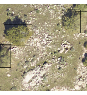
Each visible tree was annotated to create a bounding box that encompassed all portions of the vertical object. Fallen trees were not annotated. Visible standing stags were annotated.

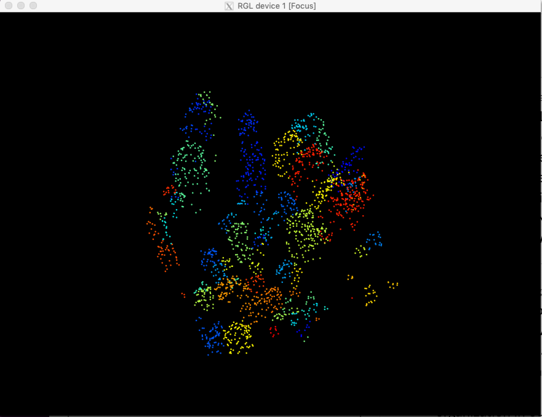
For the point cloud annotations, the two dimensional bounding boxes were draped over the point cloud, and all non-ground points (height < 2m) were excluded. Minor cosmetic cleanup was performed to include missing points. In general, the point cloud annotations should be seen as less thoroughly cleaned, given the tens of thousands of potential points in each image.

Sites (NEON locations)

siteID, State	Forest Description	Evaluation Annotations	Training Annotations
SJER, CA	Oak Savannah	462	2533
TEAK, CA	Coniferous	1483	3405
NIWO, CO	Alpine	1862	9730
MLBS, VA	Deciduous	489	1840
LENO, AL	Riparian	75	554
OSBS, FL	Southern Pine	485	1271
ABBY, OR	Coniferous	170
TALL, AL	Southern Hardwoods	93
BART, NH	Northern Hardwoods	103
BONA, AK	Riparian	272
UNDE, MI	Deciduous	134
SOAP, CA	Coniferous	115
SERC, MD	Deciduous	91
SCBI, VA	Deciduous	73
BLAN, VA	Deciduous	73
JERC, GA	Deciduous	53
HARV, MA	Northern Hardwoods	171
DSNY, FL	Southern Pine	69
CLBJ, TX	Deciduous	108
DELA, AL	Southern Hardwood	86
ONAQ, UT	Desert	25
WREF, OR	Coniferous	124

How can I add to this dataset?

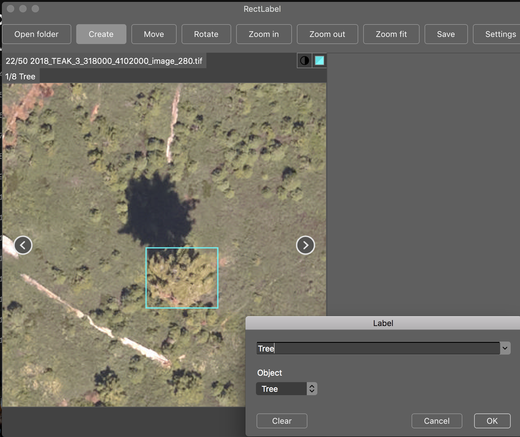
Anyone is welcome to add to this dataset by forking this repo and labeling a new site in rectlabel. For each site we have included many unannotated images. Please create a seperate folder name for your github username and send a pull request. For labeling training tiles, see the zenodo link. We recommend cropping training tiles before annotating, as all trees in an image must be annotated for training.

RGB

library(raster)
library(NeonTreeEvaluation)

#Read RGB image as projected raster
rgb_path<-get_data(plot_name = "SJER_021",sensor="rgb")
rgb<-stack(rgb_path)

#Path to dataset
xmls<-readTreeXML(siteID="SJER")

#View one plot's annotations as polygons, project into UTM
#copy project utm zone (epsg), xml has no native projection metadata
xml_polygons <- boxes_to_spatial_polygons(xmls[xmls$filename %in% "SJER_021.tif",],rgb)

plotRGB(rgb)
plot(xml_polygons,add=T)

Lidar

To access the draped lidar hand annotations, use the "label" column. Each tree has a unique integer.

library(lidR)
path<-get_data("TEAK_052",sensor="lidar")
r<-readLAS(path)
trees<-lasfilter(r,!label==0)
plot(trees,color="label")

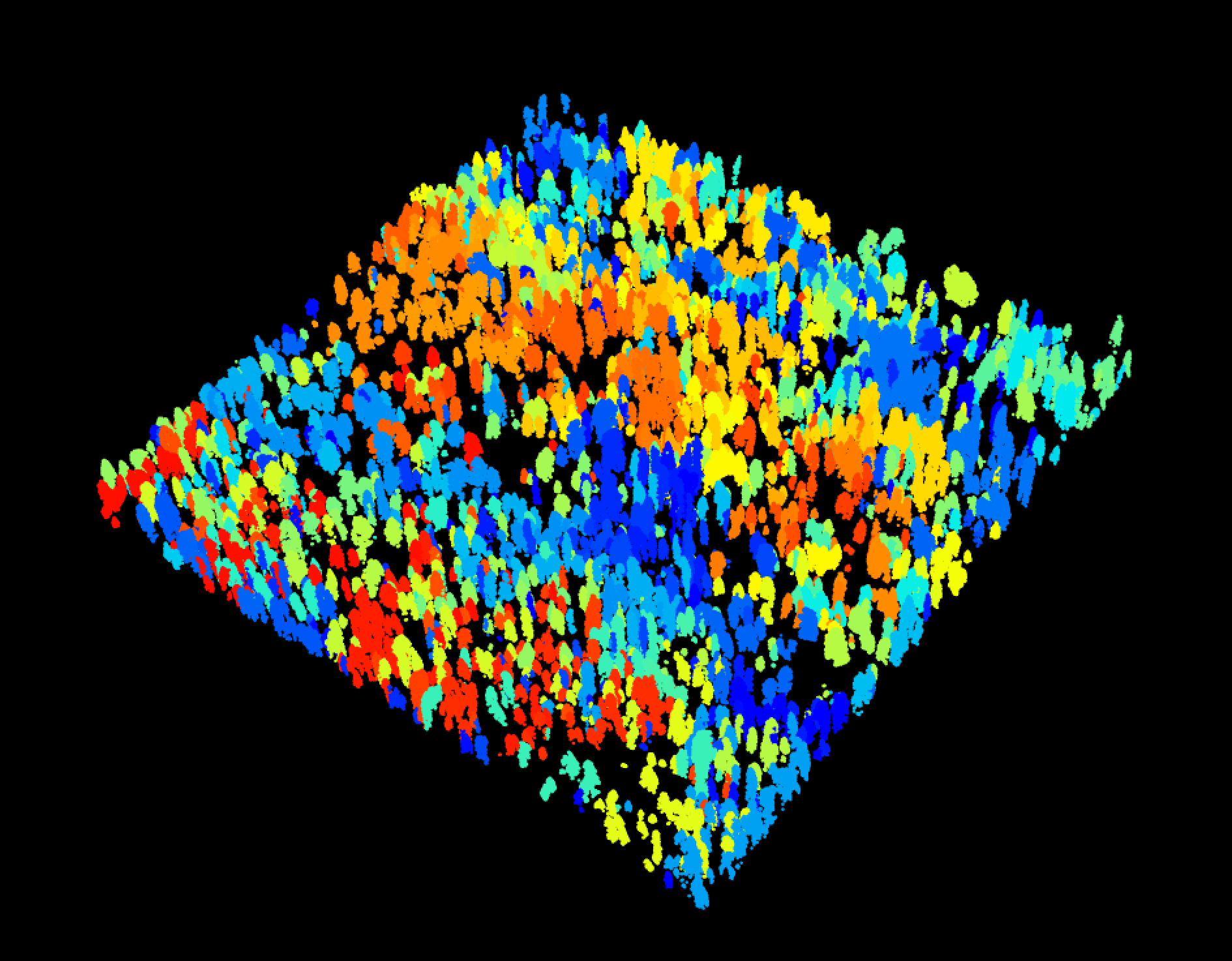
The same is true for the training tiles (see below)

We elected to keep all points, regardless of whether they correspond to tree annotation. Non-tree points have value 0. We recommend removing these points before evaluating the point cloud. Since the annotations were made in the RGB and then draped on to the point cloud, there will be some erroneous points at the borders of trees.

Hyperspectral

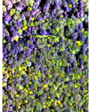
Hyperspectral surface reflectance (NEON ID: DP1.30006.001) is a 426 band raster covering visible and near infared spectrum.

path<-get_data("MLBS_071",sensor="hyperspectral")
g<-stack(path)
nlayers(g)
[1] 426
#Grab a three band combination to view as false color
g<-g[[c(17,55,113)]]
nlayers(g)
[1] 3
plotRGB(g,stretch="lin")

And in the training data:

Training Tiles

We have uploaded the large training tiles to Zenodo for download.

https://zenodo.org/record/3459803#.XpeLTVNKhQI

The annotated trainings tiles cropped for the NIWO, MLBS, SJER, TEAK, LENO, and OSBS sites. These site training tiles vary in size. These files have been cropped and saved as GEOTIFF to match RGB format.
Unannotated training tiles for the 15 additional sites. Training tiles do not overlap with evaluation plots. These have not been cropped to more reasonable hand-annotation size and are in the raw .h5 file format. For help manipulating this files, see /python_utilities/hyperspectral.py

Performance

To submit to this benchmark, please see

https://github.com/weecology/NeonTreeEvaluation_package

The primary evaluation statistic is precision and recall across all sites. It is up to the authors to choose the best probability threshold if appropriate.

Author	Precision	Recall	Description
Weinstein et al. 2019 ¹	0.55	0.65	Semi-supervised RGB Deep Learning
Silva et al. 2016	0.23	0.33	Unsupervised LiDAR raster
Dalponte et al 2016	0.23	0.34	Unsupervised LidAR raster
Li et al. 2012	0.06	0.12	Unsupervised LiDAR point cloud

To reproduce the analysis for the benchmark comparison see https://github.com/weecology/NeonTreeEvaluation_analysis

Cited

¹ Weinstein, Ben G., et al. "Individual tree-crown detection in RGB imagery using semi-supervised deep learning neural networks." Remote Sensing 11.11 (2019): 1309. https://www.mdpi.com/2072-4292/11/11/1309 Thanks to the lidR R package for making algorithms accessible for comparison.

Please submit a pull request, or contact the mantainer if you use these data in analysis and would like the results to be shown here.

brakuta/NeonTreeEvaluation