{soilmotif}

The goal of {soilmotif} is to provide an easy way to fit generalized shape functions to soil property data that vary over depth. The parameters of shape functions are designed to provide simple terminology and intuitive descriptors for comparing the depth distributions of properties found in soils of different areas and as predicted by different types of models.

Installation

You can install the development version of {soilmotif} like so:

remotes::install_github("brownag/soilmotif")

Example

This is a basic example which shows you how to fit a sigmoidal depth distribution model to a step and spline representations of some soil property data as a function of depth.

The sample data comes from the {aqp} jacobs2000 dataset. We are using just select horizon data from the first profile in that SoilProfileCollection object.

library(soilmotif)

# from aqp::jacobs2000, profile 1
x <- data.frame(
  id = "jacobs2000_1",
  top = c(0, 18, 43, 79, 130, 153, 156),
  bottom = c(18, 43, 79, 130, 153, 156, 200),
  clay = c(7, 6, 39, 41, 51, 50, 47),
  depletion_pct = c(0, 0, 0, 0, 2, 0, 15)
)

Step-wise Horizon-level Depletion Percentage Example

Common morphologic descriptions of soils by genetic horizon can be made continuous by assuming they represent a “step” function. Repeat the horizon-level property value as many times as each horizon is thick (in centimeters, or whatever unit you are interested in).

Here, we convert the percentage of the matrix occupied by depletions depletion_pct into a continuous step-function representation, then attempt to fit a sigmoid model to the distribution using sm_motif(). After inspection, we use sm_optim() to optimize a model based on our first guess (that the depletions appear around 40 cm and peak by 60 cm).

depl_step <- rep(x$depletion_pct, x$bottom - x$top)

plot(rep(c(0, 20), 100), 1:200, ylim = c(200, 0), type = "n",
     xlab = "Depletion %", ylab = "Depth, cm")
points(depl_step, 1:200, pch = "+")

# visualize what the "first guess" looks like
lines(sm_motif(depl_step, c(40, 60)), 1:200, col = "red", lty = 2)

# find an optimized model
m <- sm_optim(depl_step, c(40, 60))
lines(m, 1:200, col = "blue")
attr(m, "par")
#> [1] 156.6496 156.7814

legend("topright", c("Input", "Initial", "Optimized"),
       pch = c("+", NA, NA),
       lty = c(NA, 2, 1),
       col = c("BLACK","RED","BLUE"))

We find that the blue line (the optimized model) captures the transition, and best-fit parameters indicate a rapid increase at 156 cm depth, mirroring the increase from the input data.

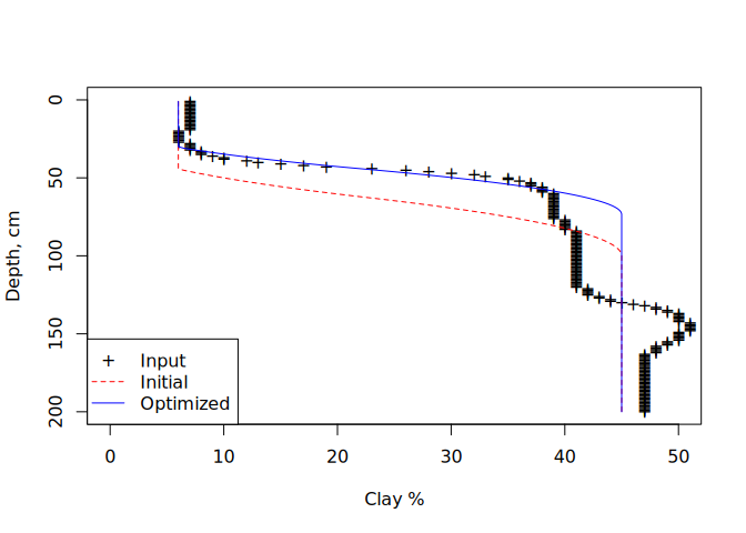
Continuous Spline Clay Content Example

The results can be more interesting when the depth function is more complicated. The simplified shapes can be used to group and generalize patterns, while ideally capturing the same types of major transitions across depth.

The following is a mass-preserving spline created using {mpspline2}, with values rounded to integers for compression into "rle" object for minimal example:

clay_spline <- inverse.rle(structure(list(
  lengths = c(19, 8, 5, 3, 1, 2, 1, 1, 1, 1, 1, 1, 1, 1, 1, 1, 1, 2, 1, 3, 4, 
              17, 7, 37, 5, 2, 2, 1, 1, 1, 2, 2, 6, 6, 6, 3, 5, 38),
  values = c(7, 6, 7, 8, 9, 10, 12, 13, 15, 17, 19, 23, 26, 28, 30, 32, 33, 35,
             36, 37, 38, 39, 40, 41, 42, 43, 44, 45, 46, 47, 48, 49, 50, 51, 50,
             49, 48, 47)), class = "rle"
))

plot(rep(c(0, 50), 100), 1:200, ylim = c(200, 0), type = "n",
     xlab = "Clay %", ylab = "Depth, cm")
points(clay_spline, 1:200, pch = "+")
lines(sm_motif(clay_spline, c(25, 100)), 1:200, col = "red", lty = 2)
m <- sm_optim(clay_spline, c(25, 100))
lines(m, 1:200, col = "blue")
attr(m, "par")
#> [1] 15.42749 73.44347

legend("bottomleft", c("Input", "Initial", "Optimized"),
       pch = c("+", NA, NA),
       lty = c(NA, 2, 1),
       col = c("BLACK","RED","BLUE"))

In this case we find that the optimized parameters result in a steeper gradient of property increase than was initially guessed with parameters c(25, 100), which had the “initial” transition centered around 63 cm. The “optimized” curve is shifted upwards by about 20 cm, with final parameters 15.4274881, 73.4434748 reflecting a smooth spline increase around 45 cm.