This is the code for my solution to the Kaggle competition hosted by Max Planck Meteorological Institute, where the task is to segment images to identify 4 types of cloud formations. It scores in the top 10%.
For the neural network I used a very standard approach, a pre-trained U-net. My main innovations were in pre-processing the training images to remove noise, and post-processing the neural network outputs to get the final prediction.
get_image_arrays.py processes the images and ground truth data. It calls functions in prepare_data.py.
train_nn4.py trains and saves the neural network. There are options for training using all the training data,
or holding out some for calibration and validation.
calibrate_and_predict.py calibrates the model on a hold-out set of the training data to find the
best threshold and predict the probability of a given image containing any pixels of a particular class.
I worked with grayscale images shrunken to 25% of original size.
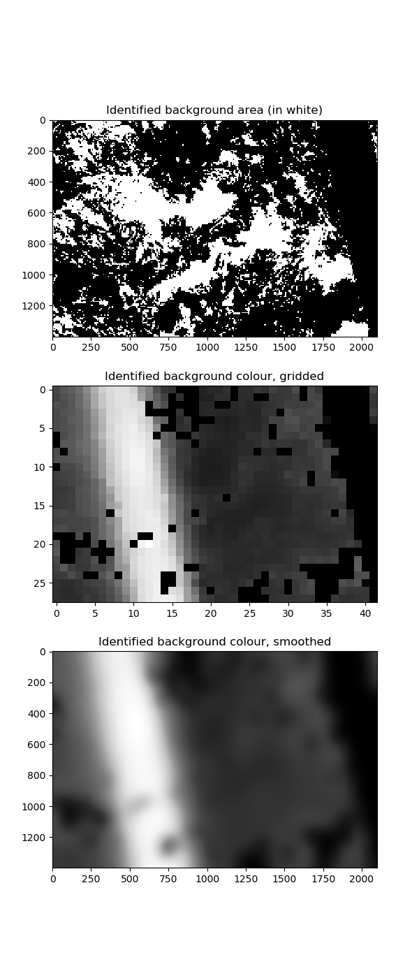
I got a large boost in model accuracy from filtering out the over-exposed areas in the images. Below is a sample image before and after correction.

I achieved this by identifying the local background colour of each part of the image. The image background is defined to
be the part of the image with small variation in pixel intensity. The parts of the image that are over-exposed have lighter
background colour. We divide the image into a grid of 50 x 50 rectangles (each rectangle having size 28 x 42 pixels).
Within each rectangle, we consider 8 x 8 pixel squares
and define a square to be in the background if its standard deviation of pixel intensity is below some threshold. We calculate
the average colour of the background in each 28 x 42 rectangle. Then we smooth the results so we get a smoothed picture
of the background colour over the whole image. Finally we rescale the image so that the range [background, 255] maps onto [0, 255].
I also changed the missing areas to a medium-grey colour. I thought this would help the neural network converge since it's more similar to the average colour of the overall images, which I thought would make the optimisation problem smoother. I'm not sure whether it made any difference.
Below is a visualisation of the steps in the correction process.
I used a blend of efficientnetb4 effecientnetb5, both pre-trained from this library: https://github.com/qubvel/segmentation_models. I trained for 10 epochs with the encoder layers frozen, then fine-tuned the whole model for 10 epochs with a lower learning rate. I did horizontal and vertical flip augmentation; I tried others but found they didn't help.
The key to post-processing is to observe that the dice metric is not continuous: if a class doesn't exist in an image, there is a huge difference in predicting 1 pixel (dice score 0) and predicting 0 pixels (dice score 1). So, to decide whether to make a non-zero prediction, we need to estimate 2 things: the probability that the class exists in the image, and the expected dice score given that the class does exist. Then we can calculate the expected dice score for a zero and a non-zero prediction, and choose between them accordingly. I built very simple models for these, all just using a single variable: the 95th percentile of the predicted class probabilities for each image. These models were built using a set of 500 images excluded from the training of the neural network model.
The optimal threshold depends on the confidence of the prediction: for more confident predictions a higher threshold is better. I tested thresholds between 0.05 and 0.95 at intervals of 0.05. For each threshold, I built a model to predict the expected dice score. This model has just one x variable, the 95th percentile prediction for the class in each image. The model is essentially just a smoothed average of the actual dice score for each x value (calculated only on the images where the class exists, because of the discontinuity of the dice metric as noted above).
When making predictions, we calculate the expected dice score for each image and threshold, then choose the best threshold. However, if the expected dice score with the optimal threshold is lower than the probability that the class exists in the image (as calculated by the model below), then we just predict all zeros.
This is similar to the above model. We use the same x variable, the 95th percentile of the pixel predictions, but this time it's a classification model, so instead of using the rolling average of the target we use a local logistic regression approach. I also used this successfully in the Santander competition; there is more detail at my github repo for that competition (https://github.com/btrotta/kaggle-santander-2019/blob/master/Readme.pdf).
I didn't attempt to reshape the predicted areas into rectangles or polygons, as in some published kernels. I also didn't enforce a minimum predicted area. My hypothesis is that this information is already built in to the neural network predictions, and that this is why augmentations that change the size or shape of the masks (e.g. skew, rotation, zoom) give poor results.