ccber: an R Package for the Estimation of Behavioral Entropy Rate - Developed for the Conte Center @ UCI
See reference: Davis, E.P., Stout, S.A., Molet, J., Vegetabile, B., Glynn, L.M., Sandman, C.A., Heins, K., Stern, H., Baram, T.Z. (2017). Exposure to unpredictable maternal sensory signals influences cognitive development across-species. Proceedings of the National Academy of Sciences. September 26, 2017. 114 (39) 10390-10395
The package devtools is required to install this R package from this
Github repository. Install this package first if it is not already
installed.
install.packages('devtools', dependencies = TRUE)
Once that package has been installed, use the following to install
ccber
devtools::install_github('bvegetabile/ccber')
Load the package to begin analysis!
library('ccber')
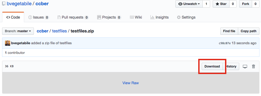
Download files from github.com/bvegetabile/ccber/tree/master/testfiles/testfiles.zip.
Navigate to the directory where the files are located using the following R command. The setwd command sets the working directory for R. ( Note in the below, the path should be changed to the location of where the files have been uncompressed )
setwd('~/git/ccber/testfiles/')
Then run the following,
test_output <- ccber::ber_analyze_dir('.')
By setting the working directory in the first step, any output files will be put in the directory specified.
If successful, you fill will see the following:
> ccber::ber_analyze_dir('.')
Completed without issue    :  Entropy_6m - 88888HE - Event Logs.xlsx
Completed without issue    :  Entropy_6m - 99999LE - Event Logs.xlsx
Script total run time:  0.013 minutes
-------------------- Check the log for files below --------------------
The object test_output contains the entropy rates and some additional
measures. The output will look as follows:
> test_output
  SubjectID CanEstimateEntropy EntropyRate
1   88888HE               TRUE   1.2755499
2   99999LE               TRUE   0.6442886
  TotalNumberOfTransitions CombinedVideoDuration PercentMissing
1                      119               600.027              0
2                       69               600.027              0
  AuditoryCounts AuditoryTotalTime AuditoryAverageTime
1             23            25.001               1.087
2             15            15.000               1.000
  VisualCounts VisualTotalTime VisualAverageTime TactileCounts
1           16        309.9636          19.37273            21
2           11        185.0270          16.82064            10
  TactileTotalTime TactileAverageTime
1         362.9628           17.28394
2         285.0273           28.50273
To save the output data to a .csv file to be read into excel later,
use the following:
write.csv(test_output,
          file = file = paste(Sys.Date(),
                              '-ber-estimates.csv',
                              sep=''),
          row.names = F)
The command Sys.Date() prepends the date to document when the data was
created
To use ccber to estimate behavioral entropy rate, see the Conte Center
website for a description of how to set up files and record
observations. The input files for these functions are described there...
To run ccber with a single file use the following function
ber_analyze_file(f_loc,
                 plot_all=F,
                 plots_to_file=F,
                 tactile_padding = 1.0,
                 auditory_padding = 1.0,
                 behavior_types=list(
                   "mom_auditory_types" = c('Vocal'),
                   "mom_tactile_types" = c('TouchBaby',
                                           'HoldingBaby'),
                   "mom_visual_types" = c('ManipulatingObject'),
                   "baby_visual_types" = c('LookAtMomActivity'),
                   "missing_types" = c('CantTellHolding',
                                       'ActivityNotVisible',
                                       'CantTellLooking')),
                 missing_threshold = 0.1)
The variables are described below:
f_loc: Location of the file to be analyzedplot_all: Logical variable to plot diagnostic plots for this individual. Defaults toFALSEplots_to_file: Logical variable which plots diagnostic plots to a file. Currently unused.tactile_padding: Padding to be applied to the "event" types of the Observer software. Padding is right-adjusted and Defaults to 1 second.auditory_padding: Padding to be applied to the "event" types of the Observer software. Padding is right-adjusted and Defaults to 1 second.behavior_types: List specifying the "auditory", "tactile", and "visual" behaviors to subset on. The "missing_types" are description of tags that define missing data.missing_threshold: Proportion value that defines what the threshold of missingness is to include the file or not. Set to 0.1 reflecting 10% of missingness is acceptable based upon the tags inbehavior_types.
To expedite processing of many files an additionally function is
provided to analyze an entire directory of Excel files. The function
ber_analyze_dir is similar to the previous function and takes as input
dir_loc.
ber_analyze_dir(dir_loc,
                tactile_padding = 1.0,
                auditory_padding = 1.0,
                behavior_types=list(
                  "mom_auditory_types" = c('Vocal'),
                  "mom_tactile_types" = c('TouchBaby',
                                          'HoldingBaby'),
                  "mom_visual_types" = c('ManipulatingObject'),
                  "baby_visual_types" = c('LookAtMomActivity'),
                  "missing_types" = c('CantTellHolding',
                                      'ActivityNotVisible',
                                      'CantTellLooking')),
                missing_threshold = 0.1,
                log_file = paste(Sys.Date(), '-ber-logfile.txt', sep=''))
The inputs that are described in the previous section are mostly same
and are passed as input to multiple calls of ber_analyze_file.
For a more detailed overview see the software description document in within the SDD folder
Consider the following transition matrix of a first-order Markov chain with three states,
P = matrix(c(0.2, 0.3, 0.5,
             0.7, 0.1, 0.2,
             0.2, 0.2, 0.6), 3,3, byrow = T)
We can simulate from a Markov process with this using the function
SimulateMarkovChain
mc_chain <- SimulateMarkovChain(trans_mat = P, n_sims = 5000)
head(mc_chain, n = 20)

##  [1] 1 2 3 3 2 1 3 1 2 3 2 1 2 3 2 1 3 1 2 1
From this we can calculate a matrix of transition counts
tc <- CalcTransitionCounts(mc_chain)
tc

##      [,1] [,2] [,3]
## [1,]  319  433  782
## [2,]  731   96  210
## [3,]  483  508 1437
And then estimate a transition matrix,
tm <- CalcTransitionMatrix(tc)
tm

##           [,1]       [,2]      [,3]
## [1,] 0.2079531 0.28226858 0.5097784
## [2,] 0.7049180 0.09257473 0.2025072
## [3,] 0.1989292 0.20922570 0.5918451
which agrees fairly well with the true P. Additionally we can estimate
the stationary distribution of the process in a one of two ways. The
first way is an empirical estimate from the observed sequence.
emp_sm <- CalcEmpiricalStationary(mc_chain, state_space = 1:3)
emp_sm

##        [,1]   [,2]   [,3]
## [1,] 0.3068 0.2074 0.4858
The second way is an eigendecomposition of the observed transition matrix, though the preferred method is through the empirical estimation procedure.
eig_sm <- CalcEigenStationary(tm)
eig_sm

## [1] 0.3066525 0.2074278 0.4859196
Using both the stationary distribution estimate and the estimate of the transition matrix, the entropy rate of the process can be estimated using the following commands
entrate1 <- CalcMarkovEntropyRate(tm, emp_sm)
entrate1

## [1] 1.36315

entrate2 <- CalcMarkovEntropyRate(tm, eig_sm)
entrate2

## [1] 1.363128
Both of these values agree very well with the true entropy rate,
true_entropy_rate <- CalcMarkovEntropyRate(P, CalcEigenStationary(P))
true_entropy_rate

## [1] 1.360979
If the method of estimation for the stationary distrbution is known, a more simple function is provided to estimate the entropy rate as well.
Both of these values agree very well with the true entropy rate,
quicker_estimate <- CalcEntropyRate(mc_chain,
                                    state_space = 1:3,
                                    stat_method = "Empirical")
quicker_estimate

## [1] 1.36315
