`gpbalancer`: an `R` Package for Optimally Balanced Gaussian Process Propensity Score Estimation

Reference forthcoming...

Installing `gpbalancer`

The package devtools is required to install this R package from this Github repository. Install this package first if it is not already installed.

install.packages('devtools', dependencies = TRUE)

Once that package has been installed, use the following to install gpbalancer

devtools::install_github('bvegetabile/gpbalancer')

Load the package to begin analysis!

library('gpbalancer')

Example using `gpbalancer`

Simulating data

Provided below is a simple simulation to explore the effectiveness of the optimally balanced Gaussian process propensity score. Consider a continuous covariate X which is used to assign treatment, for i ∈ 1, …, 1000 let,

X_i ∼ N(0, 1)

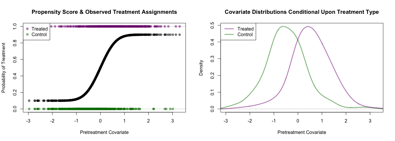
Additionally, let the true propensity score be defined as follows,

e(X_i)=Pr(T_i = 1|X_i)=0.8 × Φ(2 * X_i)+0.1

where Φ(⋅) is the cumulative distribution of the Normal Distribution. Finally, we simulate treatment assignment such that,

T_i|X_i ∼ Bernoulli( e(X_i) )

Additionally, we will consider the following potential outcomes

Y_i^T = 1 = X_i² + 2 + ϵ_i, 𝒯

Y_i^T = 0 = X_i + ϵ_i, 𝒞

where ϵ_i, G ∼ N(0, 0.25²) for G ∈ {𝒯, 𝒞}. The observed outcome will be,

Y_i^obs = I(T_i = 1)Y_i^T = 1 + I(T = 0)Y_i^T = 0

set.seed(2017)
n_obs <- 1000
pretreatment_cov <- rnorm(n_obs)
prop_score <- 0.8 * pnorm(2*pretreatment_cov) + 0.1
treatment_assignment <- rbinom(n_obs, size = 1, prob = prop_score)
ta_logical <- as.logical(treatment_assignment)
y_t <- pretreatment_cov^2 + 2 + rnorm(n_obs, sd=0.25)
y_c <- pretreatment_cov + rnorm(n_obs, sd=0.25)
y_obs <- treatment_assignment * y_t + (1-treatment_assignment) * y_c

t_col <- rgb(0.5,0,0.5,0.5)
c_col <- rgb(0,0.5,0,0.5)

Visualizing the Propensity Score & Covariate Imbalance

The true propensity score and observed treatment assignments are shown below.

par(mfrow=c(1,2))
plot(pretreatment_cov, prop_score, 
     xlim=range(pretreatment_cov), 
     ylim=c(0,1),
     pch=19, col=rgb(0,0,0,0.5),
     xlab='Pretreatment Covariate',
     ylab='Probability of Treatment',
     main='Propensity Score & Observed Treatment Assignments')
points(pretreatment_cov[ta_logical],
       treatment_assignment[ta_logical],
       pch=19, col=t_col)
points(pretreatment_cov[!ta_logical],
       treatment_assignment[!ta_logical],
       pch=19, col=c_col)
abline(h=c(0,1), lty=3)
legend('topleft', c('Treated', 'Control'), pch=19, col=c(t_col, c_col), bg='white')

plot(density(pretreatment_cov[!ta_logical], adjust = 1.5),
     xlim=range(pretreatment_cov), 
     type='l', lwd=3, col=c_col,
     xlab='Pretreatment Covariate',
     ylab='Density',
     main='Covariate Distributions Conditional Upon Treatment Type')
lines(density(pretreatment_cov[ta_logical], adjust = 1.5),
     lwd=3, col=t_col)
abline(h=c(0,1), lty=3)
legend('topleft', c('Treated', 'Control'), lty=1, lwd=3, col=c(t_col, c_col), bg='white')

knitr::kable(gpbalancer::bal_table(data.frame("Pretreatment Covariate" = pretreatment_cov), 1, ta_logical))

	NT	MeanT	VarT	NC	MeanC	VarC	StdDiff	LogRatio
Pretreatment.Covariate	494	0.5371	0.6889	506	-0.4716	0.7324	1.1966	-0.0306

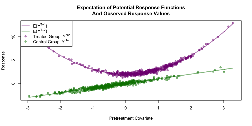
Visualizing the Potential Outcomes & Observed Responses

Below are visualizations of the expectations of the potential response functions and the observed responses for the sample data.

exes <- seq(min(pretreatment_cov), 
            max(pretreatment_cov), 
            0.01)
meanYT <- exes^2 + 2
meanYC <- exes
ylims <- range(cbind(meanYT, meanYC))

plot(exes, meanYT,
     type='l', lwd=3, col = t_col,
     xlim=range(pretreatment_cov), ylim=ylims,
     xlab='Pretreatment Covariate',
     ylab='Response',
     main='Expectation of Potential Response Functions\nAnd Observed Response Values')
lines(exes, meanYC, lwd=3, col = c_col)
points(pretreatment_cov[ta_logical], y_obs[ta_logical], pch=19, col=t_col)
points(pretreatment_cov[!ta_logical], y_obs[!ta_logical], pch=19, col=c_col)
legend('topleft', 
       c(expression(E(Y^{T==1})), 
         expression(E(Y^{T==0})),
         expression(paste('Treated Group, ', Y^{obs})), 
         expression(paste('Control Group, ', Y^{obs}))), 
       lty=c(1,1,NA,NA), lwd=c(3,3,NA,NA), pch=c(NA, NA, 19, 19), col=c(t_col, c_col), bg='white')

Under these settings if we are attempting to model τ = E(Y^T = 1 − Y^T = 0) without adjustment (i.e. using E(Y^obs|T = 1)−E(Y^obs|T = 0)), then the bias would be approximately 0.43.

hat_tau <- mean(y_obs[ta_logical]) - mean(y_obs[!ta_logical])
original_bias <- (hat_tau-3)
message('Orignal Bias: ', round(original_bias,3))

## Orignal Bias: 0.427

Estimating the Propensity Score

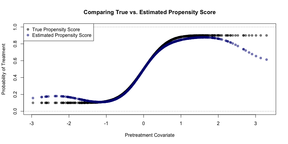
Using the above simulated data, we can now estimate the propensity score. The reported time is in seconds:

est_propscore <- gpbalancer::gpbal(X = as.matrix(pretreatment_cov), 
                                   y = treatment_assignment, 
                                   cov_function = gpbalancer::sqexp_poly,
                                   init_theta = c(1, 1),
                                   verbose = T)

## Starting Optimization  @   2019-03-07 15:54:54

## Finished Optimization  @   2019-03-07 15:55:08

## Time Difference          : 14.046

## Optimal Covariate Balance: 2e-08

Visualizing the Estimated Propensity Score

plot(pretreatment_cov, prop_score, 
     xlim=range(pretreatment_cov), 
     ylim=c(0,1),
     pch=19, col=rgb(0,0,0,0.5),
     xlab='Pretreatment Covariate',
     ylab='Probability of Treatment',
     main='Comparing True vs. Estimated Propensity Score')
points(pretreatment_cov,
       est_propscore$ps,
       pch=19, col=rgb(0,0,0.5,0.5))
abline(h=c(0,1), lty=3)
legend('topleft', c('True Propensity Score', 'Estimated Propensity Score'), pch=19, col=c(rgb(0,0,0,0.5), rgb(0,0,0.5,0.5)), bg='white')

Balance Adjusting for the True Propensity Score

true_wts <- ifelse(ta_logical, 1/prop_score, 1/(1-prop_score))
knitr::kable(gpbalancer::bal_table(data.frame("Pretreatment Covariate" = pretreatment_cov), 1, ta_logical, true_wts))

	NT	MeanT	VarT	NC	MeanC	VarC	StdDiff	LogRatio
Pretreatment.Covariate	494	-0.0569	1.0578	506	0.1781	1.1307	-0.2247	-0.0334

Balance Adjusting for the Estimated Optimally Balanced Gaussian Process Propensity Score

est_wts <- ifelse(ta_logical, 1/est_propscore$ps, 1/(1-est_propscore$ps))
knitr::kable(gpbalancer::bal_table(data.frame("Pretreatment Covariate" = pretreatment_cov), 1, ta_logical, est_wts))

	NT	MeanT	VarT	NC	MeanC	VarC	StdDiff	LogRatio
Pretreatment.Covariate	494	0.0256	0.9638	506	0.0255	0.964	1e-04	-1e-04

Evaluating the Performance of the Optimally Balanced Gaussian Process Propensity Score

We now compare the method when there is no adjustment on the propensity score and when there is adjustment by the true propensity score. To compare these three scenarios the bias, the percent reduction in bias compared with no adjustment, and the mean squared error of the estimators are provided.

	Est. ATE	S.E.	Lower95	Upper95	Bias	% Red. in Abs. Bias	MSE
No Adjustment	3.427	0.075	3.280	3.574	0.427	-	0.188
True Propensity Score	2.877	0.111	2.660	3.095	-0.123	71.242	0.027
Opt Bal GP Prop Score	2.932	0.100	2.735	3.129	-0.068	84.089	0.015

bvegetabile/gpbalancer

gpbalancer: an R Package for Optimally Balanced Gaussian Process Propensity Score Estimation

Installing gpbalancer

Example using gpbalancer