Tabular method (Quine-McCluskey method) solver - 2020-01 Digital Logic Design 01
ABSTRACT
This project was created as a part of the assignment for Digital Logic Design class 01. In this project, I implemented the Tabular Method (as known as QMM - Quine-McCluskey Method) using C++ to automate the circuit optimization process. And also In that process, I tried to lower the time complexity as much possible as I can such as implementing the search space reduction method rather than just searching for every possible combination. But even if implementing such techniques, it doesn't help in lowering the time complexity since the last step of QMM is ultimately the Set Cover problem which is NP-Complete. So I tried not only lowering the time complexity of the front part of steps in QMM or implementing techniques like search space reduction but also tried to lower the complexity of the last step which is can be seen as the Set Cover problem by sacrificing true solution. One method that was implemented in this project to accomplish this is getting an approximation solution that returns a solution that has the almost same cost as a true solution of the problem while working in a much faster time (In polynomial time). Of course, this project provides an algorithm for getting true solutions not only an approximation algorithm. At last, I tested the accuracy and performance(Runtime, Cost of the solution) of the algorithm.
- 1. Author
- 2. Version and Compile
- 3. How to use
- 4. How it works
- 5. Accuracy of the algorithm
- 6. Performance Test
- Name: 윤상건 (Sang-geon Yun)
- Student ID: 20191632
- Version: C++14
- Compile command:
g++ -std=c++14 main.cpp -o main
You can run the Tabular Method Solver using main.cpp by editing data in textCases.txt file.
The format of textCases.txt is the same as follows:
(Number of test cases)
(Number of minterms of test case #1) (Minterms)
(Number of don't cares of test case #1) (Don't cares)
(Number of minterms of test case #2) (Minterms)
(Number of don't cares of test case #2) (Don't cares)
(Number of minterms of test case #3) (Minterms)
(Number of don't cares of test case #3) (Don't cares)
...
An example of testCases.txt:
5
5 0 1 5 6 7
0
5 0 1 2 3 7
0
8 0 2 5 6 7 8 9 13
3 1 12 15
8 0 4 8 10 11 12 13 15
0
10 0 2 3 4 6 7 9 11 13 15
0
You can also run the Tabular Method Solver manually by using TabularMethodSolver.h header which supports a class for solving tabular method problems.
Checkout the following example:
vector<unsigned long long int> minterms = {0, 2, 5, 6, 7, 8, 9, 13};
vector<unsigned long long int> dontcares = {1, 12, 15};
Tabular tabular(minterms, dontcares);
cout << "True solution: " << tabular.solve(false) << endl;
cout << "Approximation: " << tabular.solve(true) << endl;
Constructor of Tabular class
Tabular::Tabular(vector<unsigned long long int>& mins, vector<unsigned long long int>& donts);mins: A vector that is containing mintermsdonts: A vector that is containing don't cares
solve method
string Tabular::solve(bool approx, bool showProcess=false);approx: if it's true,solvewill return approximate solutionshowProcess: if it's true,solvewill print process(PIs, EPIs) on standard out stream
If the number of minterms is too big to get a true solution, you can get an approximation solution that has polynomial time complexity by following.
- True solution:
tabular.solve(false) - Approximation solution:
tabular.solve(true)
Note: Every time complexities that are written in this section are approximated. So they could be not accurate.
It only can get the solution for a situation where the number of variables is less or equal to 64 since it handles minterms by unsigned long long int type.
The overall algorithm of the Tabular Method Solver can be described as the following pseudocode
string solve(bool approx){
    getPI(); // Getting Prime Implicants
    getEPI(); // Getting Essential Prime Implicants
    vector<int> ans; // Stores PIs that cover every minterm in minimum cost
    if(approx) // Finding approximation solution using PIs that are not EPI.
        ans = approximationSolver();
    else // Finding a true solution using PIs that are not EPI.
        ans = trueSolver();
    for(int i = 0, v = 0; i < PIs.size(); ++i)
        if(PIs[i].getEPI())
            ans.push_back(i); // Adding EPI to solution
    sort(ans.begin(), ans.end()); // For normalizing the solution
    string eq = ansToString(ans);  // Converting solution (PIs) to expression
    return eq; // Returing solution for input
}The algorithm that is used for getPI() is the same as the first step of the Quine–McCluskey algorithm.
Time complexity can be calculated by following when B denotes the maximum number of bits of MST among the minterms and don't cares, N denotes the number of minterms, M denotes the number of don't cares, and T_i denotes the set of numbers with the number of 1s in bits is equal to i.
- Time complexity:
O(B * sum(|T_i| * |T_(i+1)|))=O(B(N + M)^2)
When getPI() is executed, it's time to get all the EPI (Essential Prime Implicants) which are the PI that covers minterms that not be covered by any other PIs.
First of all, we need to uniform the coordinates. In this situation, the coordinate means the value of minterms. For example, if given minterms are {0, 2, 5, 6, 7, 8, 9, 13} then we can convert them into this: {0: 0, 2: 1, 5: 2, 6: 3, 7: 4, 8: 5, 9: 6, 13: 7} so we can handle minterms much easier.
This is called Coordinate Compression. And it cost O((N + M)log(N + M)) time.
After that, we can define the following tables.
cnt[i] = Number of times when coordinate i was selected by different PIs
last[i] = Index of PI that selected coordinate i in last time
We can fill up those tables in O((N + M)^2 log(N + M)) time.
Then, we can find every EPIs by following:
for(int i = 0; i < minterms.size(); ++i){
    int compPos = comp[minterms[i]]; // Compressed coordinate
    if(cnt[compPos] == 1){ // cnt[i] == 1 means the number of PIs that selected coordinate i is one (It means, there is only one PI that covers i)
        if(PIs[last[compPos]].getEPI()) // Already EPI
            continue;
        PIs[last[compPos]].setEPI(); // EPI Found!
        ++totNumberOfEPI;
    }
}
And the time complexity of above procedure is O((N + M)log(N + M))
As a result the total time complexity of getEPI() is:
- Time complexity:
O((N + M)log(N + M) + (N + M)^2 log(N + M) + (N + M)log(N + M))=O((N + M)^2 log(N + M))
First of all, we know that EPIs must be chosen since there are no other PIs that cover certain coordinates.
So, we can eliminate EPIs and coordinates that are chosen by those EPIs from the problem.
And then, we need to choose a minimum number of PIs among the rest of the PIs.
This is where the problem gets really difficult.
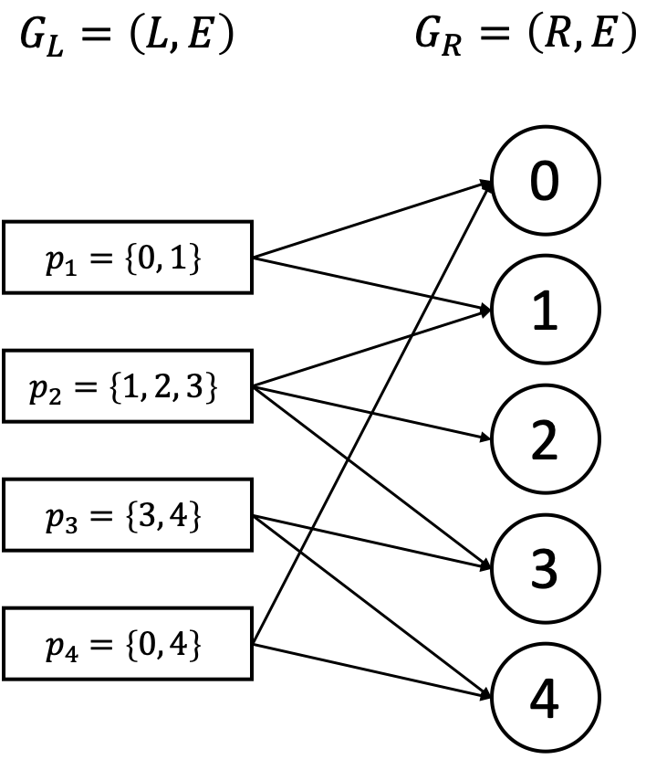
Let's say we got the following PIs:
p1 = {0, 1}
p2 = {1, 2, 3}
p3 = {3, 4}
p4 = {0, 4}
And we have to cover {0, 1, 2, 3, 4} by choosing the PIs that are listed above.
To make this problem easier to see, we can make the graph as follows:
Now, the problem is converted to Set Cover Problem since we have to choose a minimum number of vertices from G_L to flow from G_L to every vertex in G_R.
And as you know, the Set Cover problem is the NP-complete problem. So, it's impossible to find a true solution in polynomial time.
So, I made two ways to solve this problem. By Brute force Algorithm with reducing search space technique and Greedy Algorithm using max segment tree.
4.2.4.1. Algorithm for getting true solution: Brute force Algorithm with reducing search space technique
The code for this is the same as follows:
void bruteForce(vector<vector<int>>& G, vector<int>& selected, vector<int>& nowCase, vector<int>& minCase , int selCnt, int idx, int cost, int& minCost){
    if(idx == G.size() || (minCost != -1 && minCost <= cost)) // Reducing search space using current minimum solution
        return;

    // search without choosing the current vertex
    bruteForce(G, selected, nowCase, minCase, selCnt, idx + 1, cost, minCost);

    // search while choosing the current vertex
    int cnt = 0;
    for(int i = 0; i < G[idx].size(); ++i){
        int u = G[idx][i];
        if(!selected[u]) ++cnt;
        ++selected[u];
    }
    nowCase.push_back(idx);
    if(cnt){ // Check if choosing current vertex made new selected vertex in G_R
        if(selCnt + cnt == selected.size()){ // If every vertices in G_R are selected
            if(minCost == -1 || minCost > cost + 1){ // Update minimum cost
                minCost = cost + 1;
                minCase.clear();
                for(int i = 0; i < nowCase.size(); ++i)
                    minCase.push_back(nowCase[i]);
            }
        }else{
            bruteForce(G, selected, nowCase, minCase, selCnt + cnt, idx + 1, cost + 1, minCost);
        }
    }
    for(int i = 0; i < G[idx].size(); ++i){
        int u = G[idx][i];
        --selected[u];
    }
    nowCase.pop_back();
}
It simply does the DFS(Depth First Search) for every possible case based on the current minimum cost. So, it has exponential time complexity.
- Time complexity:
O(2^(N + M) + N + M)
As you saw in 4.2.4.1. it is impossible to solve for a true solution when the number of minterms gets higher.
So, it is much more realistic to solve this Set Cover problem in polynomial time by getting an approximation solution.
My idea on this approximation solution is like the following pseudocode:
Count := number of selected vertices in G_R
Flow[v] := number of unselected vertexes in G_R that vertex v from G_L is directing
while Count < |G_R|:
    v := argmax(Flow)
    Select v
    Add v to solution
    Update Flow[]
It is a simple method but, getting the value of argmax(Flow) and updating Flow[] consume a lot of time.
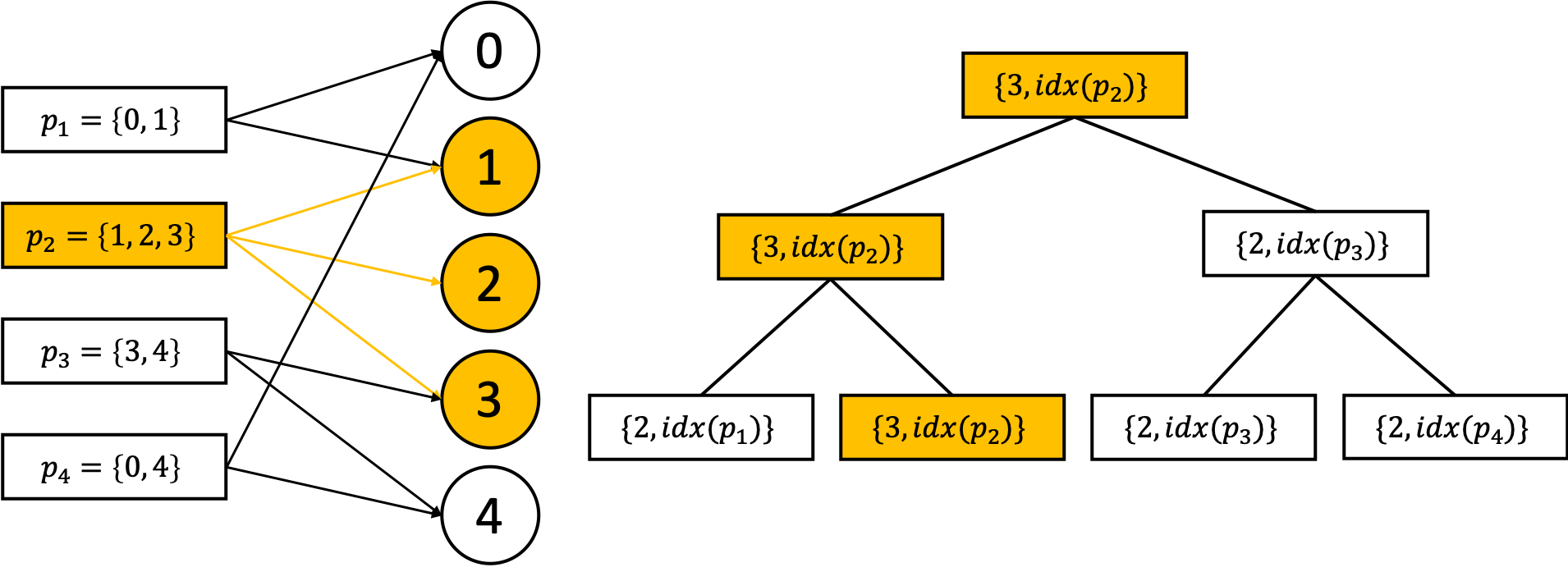
To make getting the value of argmax(Flow) and updating Flow[] faster, I used Max Segment Tree.
Each node in the segment tree is constructed by the following structure:
struct segNode{
    int value, idx;
    segNode(){
        value = -1; idx = -1;
    }
    segNode(int value, int idx){
        this->value = value;
        this->idx = idx;
    }
    bool operator<(const segNode& another)const{
        return value < another.value;
    }
    bool operator>(const segNode& another)const{
        return value > another.value;
    }
    segNode operator+(const segNode& another)const{
        segNode ret;
        ret.value = value + another.value;
        ret.idx = idx;
        return ret;
    }
};
Each node has two values:
value: number of unselected vertexes in G_R that vertex v from G_L is directingidx: index of a vertex inG_L
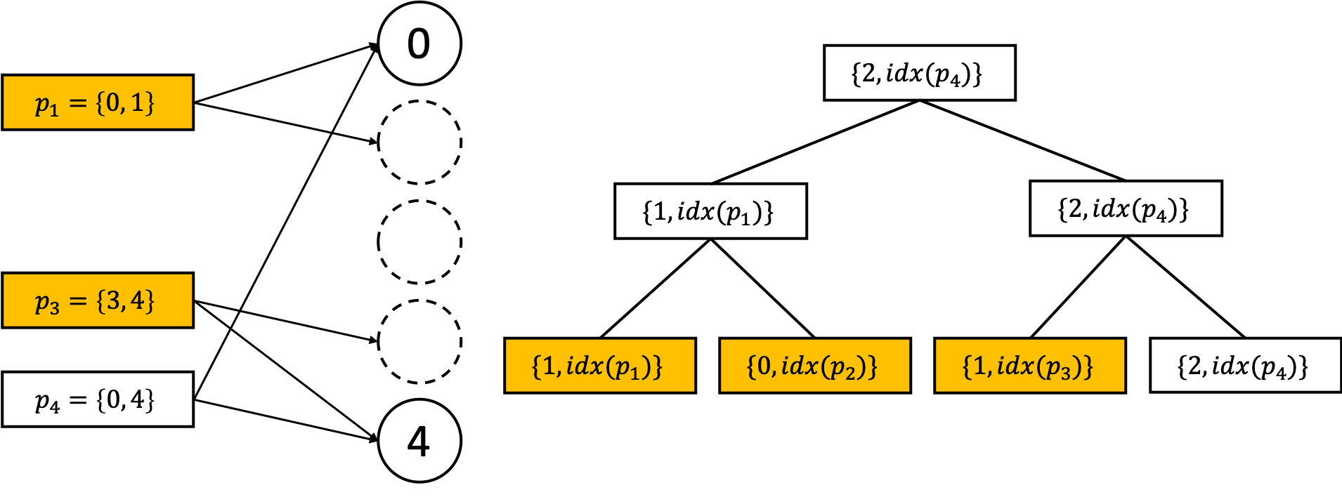
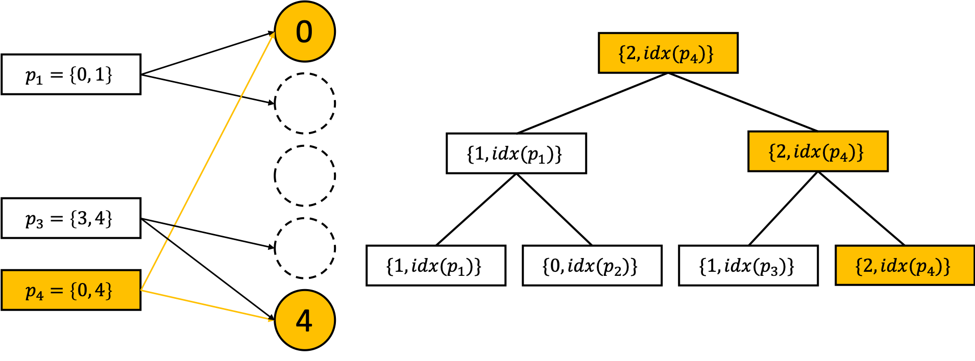
Using this segment tree, we can perform getting the value of argmax(Flow) in O(log(N + M)) and updating Flow[] in O(log(N + M)) (Amortized time complexity).
Checkout the following example:
- Getting
argmax(Flow)
- Updating
Flow[]
- Getting
argmax(Flow)
A full greedy algorithm using a segment tree written in C++ is the same as the following:
void greedy(vector<vector<int>>& GL, vector<vector<int>>& GR, vector<int>& selected, vector<int>& minCase){
    int nL = GL.size(), nR = GR.size();
    MaxSegment<segNode> seg(nL);
    for(int v = 0; v < nL; ++v)
        seg.setValue(0, v, 0, nL - 1, segNode(GL[v].size(), v));

    int count = 0;
    while(count < selected.size()){
        segNode maxnode = seg.query(0, 0, nL - 1, 0, nL - 1);
        minCase.push_back(maxnode.idx);
        for(int i = 0; i < GL[maxnode.idx].size(); ++i){
            int u = GL[maxnode.idx][i];

            if(selected[u]) continue;
            selected[u] = true;
            ++count;
            for(int j = 0; j < GR[u].size(); ++j){
                int v = GR[u][j];

                seg.update(0, v, 0, nL - 1, segNode(-1, 0));
            }
        }
    }
}
Unfortunately, the code above has one problem. For each of the vertices in G_R, it is guaranteed to visit only one-time thanks to if(selected[u]) continue;. But, to check whether the vertex has been visited or not, selected[u] should be checked every time when G_L has an edge to vertex u so, one vertex can be visited multiple times.
To solve this, I implemented an Ordered Balanced Tree aka std::set. The following code shows a new object called GLSet. Using this, we can manage each of the vertices much more efficiently by removing edges that flow to selected vertices in G_R from each of the vertices in G_L to prevent multiple times visiting.
void greedy(vector<vector<int>>& GL, vector<vector<int>>& GR, vector<int>& minCase){
    int nL = GL.size(), nR = GR.size();
    MaxSegment<segNode> seg(nL);
    for(int v = 0; v < nL; ++v)
        seg.setValue(0, v, 0, nL - 1, segNode(GL[v].size(), v));

    vector<set<int>> GLSet(GL.size());
    for(int i = 0; i < GL.size(); ++i)
        GLSet[i] = set<int>(GL[i].begin(), GL[i].end());

    int count = 0;
    while(count < GR.size()){
        segNode maxnode = seg.query(0, 0, nL - 1, 0, nL - 1);
        minCase.push_back(maxnode.idx);
        for(auto itr = GLSet[maxnode.idx].begin(); itr != GLSet[maxnode.idx].end(); ++itr){
            int u = *itr;
            ++count;
            for(int i = 0; i < GR[u].size(); ++i){
                int v = GR[u][i];
                if(v != maxnode.idx)
                    GLSet[v].erase(u);
                seg.update(0, v, 0, nL - 1, segNode(-1, 0));
            }
        }
        GLSet[maxnode.idx].clear();
    }
}- Time complexity:
O(N log(N))(Amortized time complexity)
The approximate time complexities of each method are:
- True Solution:
O(2^(N + M)) - Approximation Solution:
O((N + M)^2 log(N + M))
I tested the accuracy of the algorithm using the following test cases:
5
5 0 1 5 6 7
0
5 0 1 2 3 7
0
8 0 2 5 6 7 8 9 13
3 1 12 15
8 0 4 8 10 11 12 13 15
0
10 0 2 3 4 6 7 9 11 13 15
0
And the result is this:
Minterms: 0, 1, 5, 6, 7,
Dont cares:
# Getting PI(s)...
Number of PIs: 4
00-: {0, 1}
-01: {1, 5}
1-1: {5, 7}
11-: {6, 7}
# Getting EPI(s)...
Number of EPIs: 2
00-: {0, 1}
11-: {6, 7}
# Getting Solution...
True solution: F = a'b' + ac + ab
Approximation: F = a'b' + ac + ab

Minterms: 0, 1, 2, 3, 7,
Dont cares:
# Getting PI(s)...
Number of PIs: 2
-11: {3, 7}
0--: {0, 1, 2, 3}
# Getting EPI(s)...
Number of EPIs: 2
-11: {3, 7}
0--: {0, 1, 2, 3}
# Getting Solution...
True solution: F = bc + a'
Approximation: F = bc + a'

Minterms: 0, 2, 5, 6, 7, 8, 9, 13,
Dont cares: 1, 12, 15,
# Getting PI(s)...
Number of PIs: 7
00-0: {0, 2}
0-10: {2, 6}
011-: {6, 7}
-00-: {0, 1, 8, 9}
1-0-: {8, 9, 12, 13}
--01: {1, 5, 9, 13}
-1-1: {5, 7, 13, 15}
# Getting EPI(s)...
Number of EPIs: 0
# Getting Solution...
True solution: F = a'cd' + b'c' + bd
Approximation: F = a'cd' + b'c' + bd

Minterms: 0, 4, 8, 10, 11, 12, 13, 15,
Dont cares:
# Getting PI(s)...
Number of PIs: 6
10-0: {8, 10}
101-: {10, 11}
110-: {12, 13}
1-11: {11, 15}
11-1: {13, 15}
--00: {0, 4, 8, 12}
# Getting EPI(s)...
Number of EPIs: 1
--00: {0, 4, 8, 12}
# Getting Solution...
True solution: F = ab'c + abd + c'd'
Approximation: F = ab'c + abd + c'd'

Minterms: 0, 2, 3, 4, 6, 7, 9, 11, 13, 15,
Dont cares:
# Getting PI(s)...
Number of PIs: 4
0--0: {0, 2, 4, 6}
0-1-: {2, 3, 6, 7}
--11: {3, 7, 11, 15}
1--1: {9, 11, 13, 15}
# Getting EPI(s)...
Number of EPIs: 2
0--0: {0, 2, 4, 6}
1--1: {9, 11, 13, 15}
# Getting Solution...
True solution: F = a'd' + cd + ad
Approximation: F = a'd' + cd + ad
True solution means a solution that used the DFS method which is designed to guarantee the true solution (minimum possible cost solution). Meanwhile, Approximation means a solution that used the greedy method.
In this section, we're going to check how well the algorithm works from two perspectives: runtime, and cost of the solution.
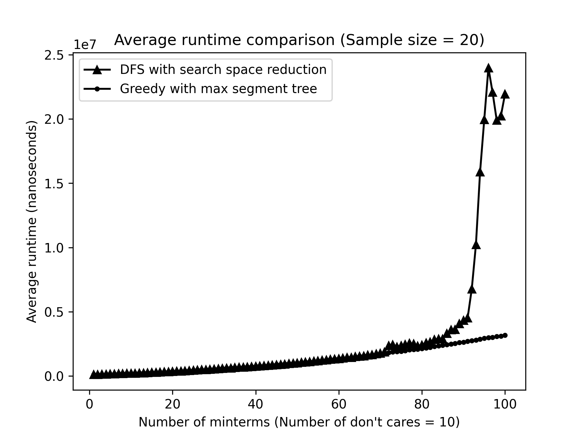
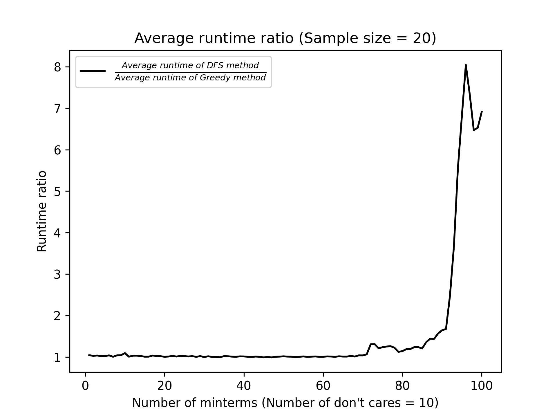
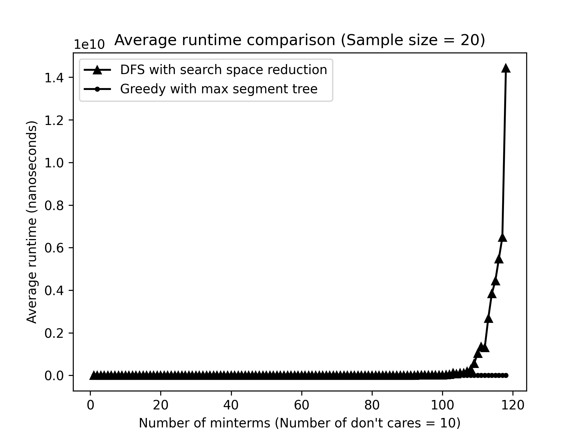
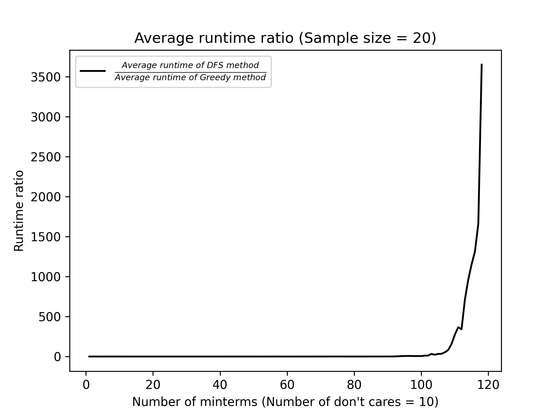
The main point is comparing the results of two methods which are DFS with search space reduction, and greedy algorithm with max segment tree.
To measure indexes(Runtime, and cost of the solution) of the algorithm, I set the sample size as 20. It means that measures 20 (sample size) times for a single constraint(In this case, the number of minterms) and then stores the arithmetic mean of those measured 20 values which is representing a measured value of the index for a single constraint.
Input data was generated in uniform random. And for uniformed input data, I made ith sample in each constraint using ith random seed. It means that samples in the same order in each constraint will have the same random seed.
You can find the code used in these tests in the ./test directory.
You can notice that the runtime of the DFS method increases on the exponential scale while the runtime of the greedy method increases on the polynomial scale. Especially in the last case (Number of minterms = 118) DFS method was 3,651 times slower than the Greedy method.
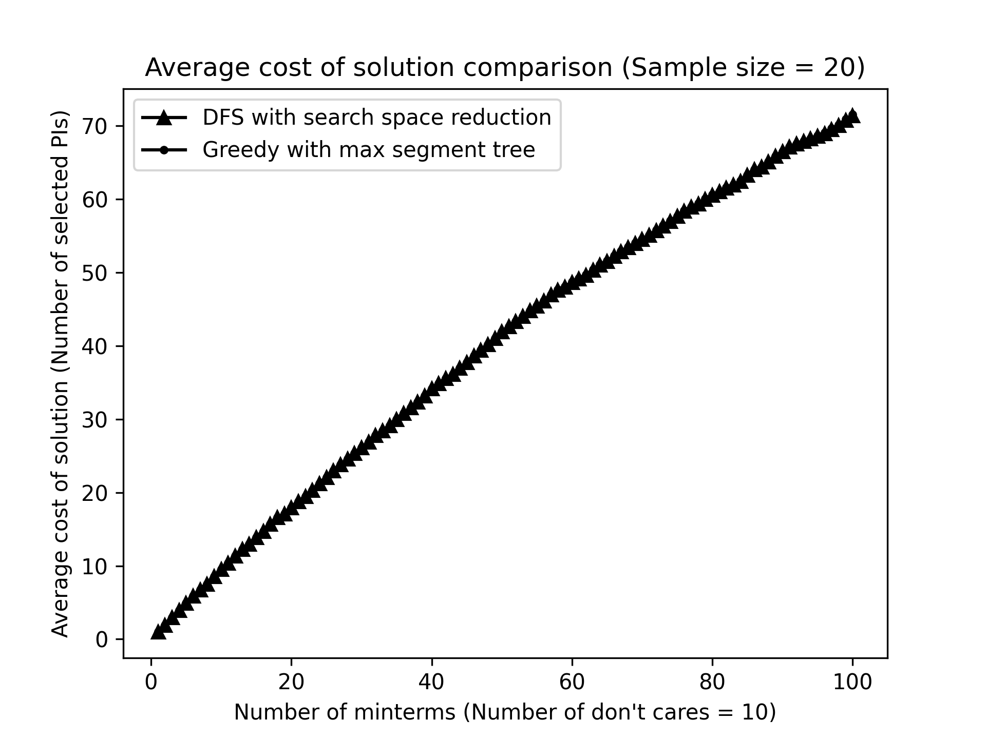
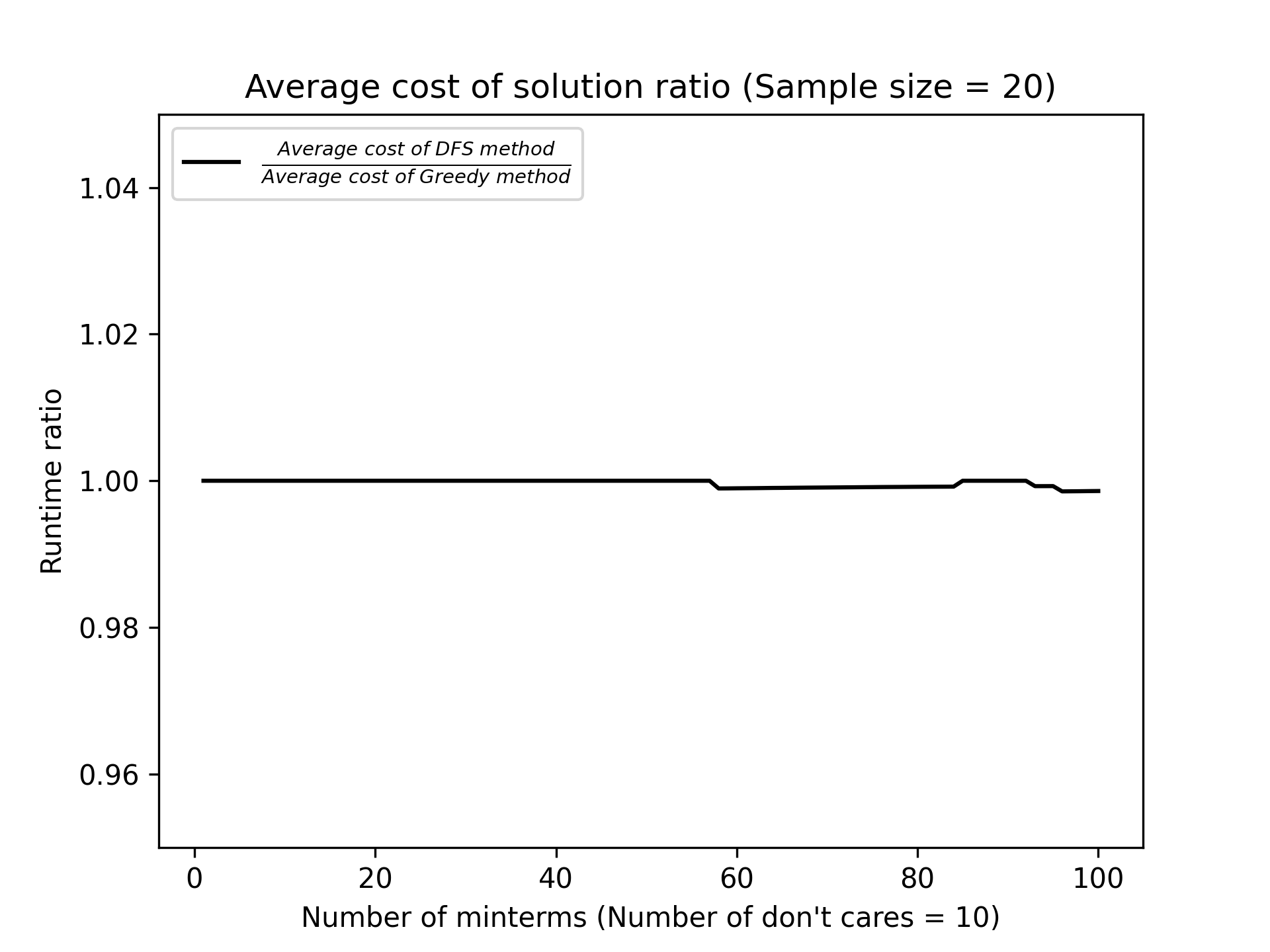
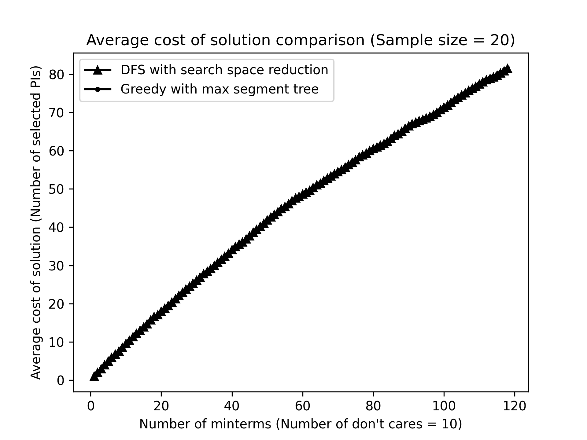
Cost means the number of PIs that are selected to cover all the given minterms.
The ratio of the average cost of solution almost equals the value of 1 even though the ratio of average runtime gets much much larger.
