pdefourier: A package for doing Fourier analysis and solving partial differential equations in Maxima CAS

Fourier analysis provides a set of techniques for solving partial differential equations (PDEs) in both bounded and unbounded domains, and various types of initial conditions. In the bounded domain case, the method of separation of variables leads to a well-defined algorithm for developing the solution in a Fourier series, making this problem tractable with a CAS.

Overview
Installation
Fourier coefficients and series
Frequency spectrum
The heat equation
The wave equation
The Laplace equation
Bessel functions

Overview

This Maxima package computes symbolically the Fourier of piecewise-smooth functions. Using the method of separation of variables it is also able to symbolically solve the one-dimensional heat and wave equations on a domain [0,L], with regular Sturm-Liouville conditions, that is, general boundary conditions of the form:

α₁u(0,t) + β₁u_x(0,t) = h₁(t)
α₂u(L,t) + β₂u_x(L,t) = h₂(t)

Moreover, the package can solve the two-dimensional Laplace equation for a variety of domains (rectangles, disks, annuli, wedges) either with Dirichlet or Neumann boundary conditions. In the case of a rectangular domain [0,a] x [0,b], the package can solve the Laplace equation with mixed boundary conditions of the form

(1-α)u(x,0) + αu_y(x,0) = f₀(x), 0 ≤ x ≤ a
(1-β)u(x,b) + βu_y(x,b) = f_b(x), 0 ≤ x ≤ a
(1-γ)u(0,y) + γu_x(0,y) = g₀(y), 0 ≤ y ≤ b
(1-δ)u(a,y) + δu_x(a,y) = g_a(y), 0 ≤ y ≤ b

where α,β,γ,δ ∈ {0,1}.

Of course, in all cases it is possible to truncate a series to make numerical calculations.

Remark: pdefourier automatically loads other packages, including piecewise, draw, simplify_sum, and syntactic_factor. The Maxima package syntactic_factor was written by Stavros Macrackis. Currently, pdefourier loads the files piecewise and syntactic_factor contained in this repository.

The Documentation folder folder contains a pdf file explaining some technical details of the implementation and a description of many of the functions contained in the package, as well as their syntax. Also, there is a Maxima session (in wxm format) with lots of examples, graphics, animations and tips for use. Here, we only give a quick introduction to the main commands used for solving typical problems.

Installation

The package can be installed by putting a copy of the files pdefourier.mac, syntactic_factor.mac, and piecewise.mac inside a folder contained in the environment variable file_search_maxima. In a Linux box, such a system-wide location could be something like /usr/share/maxima/5.42.2/share/contrib/, while in a Windows environment typically it will be c:\Program files (x86)\Maxima-sbcl-5.42.0/share/maxima/5.42.0/share/contrib (you may need administrator rights in order to do that in either case). The package can then be loaded with the command load(pdefourier) inside a Maxima session.

Fourier coefficients and series

The package can deal with piecewise functions, defined in natural notation:

(%i1) load("pdefourier.mac")$
(%i2) v(x):=if (-%pi<=x and x<0) then x^2 elseif (0<=x and x<=%pi) then sin(3*x)$

It is possible to detect the parity of such a functions, with paritycheck; possible outcomes are even, odd or none:

(%i3) paritycheck(v(x),x);
(%i2) none

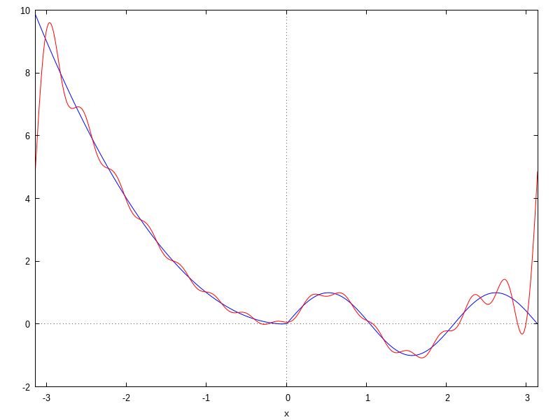
Let us draw the curve to chek the answer:

(%i4) plot2d(v(x),[x,-%pi,%pi],[ylabel,"v(x)"]);
(%t4)

The Fourier coefficients are computed with fouriercoeff, whose syntax is

fouriercoeff(expr,var,p)

Here p=(b-a)/2 if the whole interval of definition for expr is [a,b]. The output has the form

[[a₀,a_n,b_n],svlist]

where svlist is a sublist containing the singular values of the coefficients, again with the format

[m,a_m,b_m]

In the example we are considering, notice that the function is defined on [-ππ]:

(%i5) fouriercoeff(v(x),x,%pi);

This example illustrates the presence of singular values of the coefficients (for n=3). We can approximate the function by its Fourier series truncated to order 15:

(%i6) vseries15:fourier_series(v(x),x,%pi,15)$
(%i7) wxplot2d([v(x),vseries15],[x,-%pi,%pi],[legend,false]);
(%t7)

Here is a well-known example of an unbounded function:

(%i8) absolute(x):=if (x<=0) then -x elseif (x>0) then x$
(%i9) paritycheck(absolute(x),x);
(%o9) even

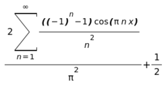
and its bounded version, for which we compute the Fourier series:

(%i10) absolute0(x):=if ( x>=-1 and x<=0) then -x elseif (x>0 and x<=1) then x$
(%i11) paritycheck(absolute0(x),x);
(%o11) even
(%i12) fourier_series(absolute0(x),x,1,inf);

Frequency spectrum

Frequency analysis is very useful in Engineering applications (but also in Physics). This technique requires that the Fourier series be first re-expressed using the identity

a cos(w)+b sin(w)=r cos(w-u)

where the modulus and the phase shift are given, respectively, by r=sqrt(a²+b²) and u=atan(b/a). Then, we can rewrite the terms of the series in the so-called harmonic form:

c_n cos(nwx-u_n)

In the theory of sound, the first harmonic (corresponding to n=1) is called the fundamental harmonic. The remaining ones are called overtones. The coefficients c_n are the harmonic amplitudes, and the absolute value |c_n| is a measure of the relative importance of the nth harmonic in a given signal (sound). The frequency analysis is done in pdefourier with the aid of the function fourier_freq. The function fourier_harm returns a list with the first n harmonics of a given function, with the syntax

fourier_harm(function(variable),variable,p,n)

where p=(b-a)/2 and [a,b] is the interval of definition of the function, while fourier_freq_list (with the same syntax) gives the list of the amplitudes.

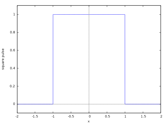
Here is the example of the square pulse with compact support on [-2,2]:

(%i1) load(pdefourier)$
(%i2) square0(x):=if (-2<=x and x<-1) then 0 elseif (-1<=x and x<=1) then 1 elseif (1 < x and x< =2) then 0$
(%i3) plot2d(square0(x),[x,-2,2],[y,-0.1,1.1],[ylabel,"square pulse"]);
(%t3)

(%i4) fourier_harm(square0(x),x,2,5);

(%i5) fourier_freq_list(square0(x),x,2,5);
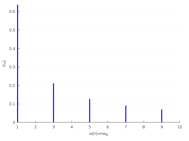
(%o5) [[1.0,0.6366197723675814],[2.0,0.0],[3.0,0.2122065907891938],[4.0,0.0],[5.0,0.1273239544735163]]

For smooth or mildly non-smooth functions, the Fourier series converges very fast, and so the first few terms suffice to get a good approximation. This is reflected in the relative weight of each harmonic (fastly decreasing), and can be visualized (using the wxMaxima frontend) with the command wxfourier_freq:

(%i6) wxfourier_freq(square0(x),x,2,10);
(%t6)

For very discontinous functions, the amplitude of harmonics does not decrease that fast (or does not decrease at all). Consider the following function as an example:

(%i7) f0(x):=if (x>=-4 and x<-3 ) then 0 elseif (-3<=x and x<=-2) then 1 elseif (-2=3 and x<=4) then 0$

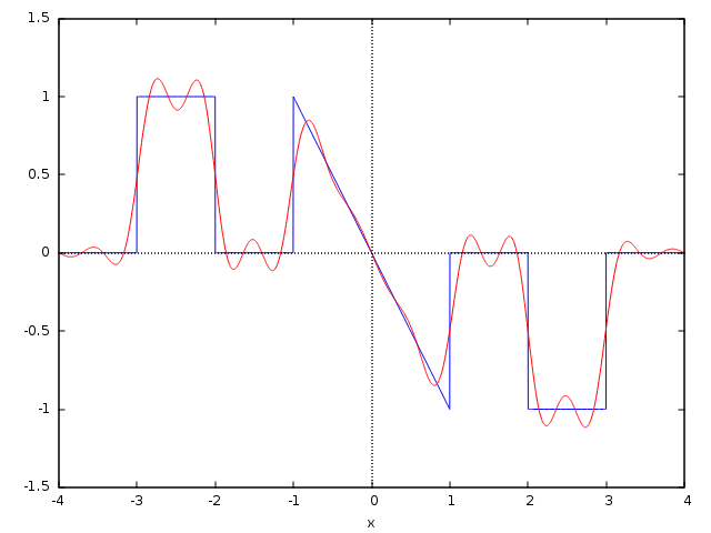
Here is its graphical representation, along with its Fourier approximation up to order 15:

(%i8) seriesf0:fourier_series(f0(x),x,4,15)$
(%i9) plot2d([f0(x),seriesf0],[x,-4,4],[legend,false]);
(%t9)

And its frequency spectrum (containing the first 10 harmonics):

(%i10) wxfourier_freq(f0(x),x,4,10);
(%t10)

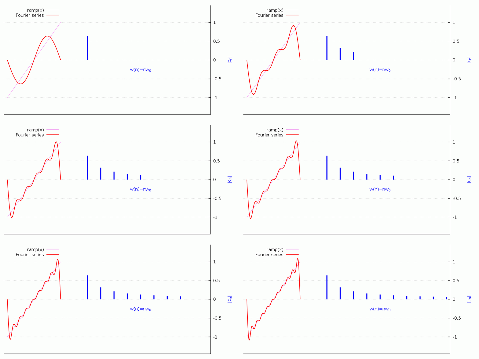
Finally, notice that adding terms to the Fourier series reflects in the harmonic content of the signal, as the following animation shows (this too requires the wxMaxima frontend):

(%i11) ramp(x):=if (-5<=x and x<=-1) then (x+3)/2 else 0$
(%i12) define(ramp_series(x,n),fourier_series(ramp(x),x,2,n))$

(%i13)	with_slider_draw(k,makelist(j,j,1,10),
    dimensions=[900,450],
    xrange=[-5.25,10.25],
    yrange_secondary=[-1.45,1.45],
    axis_top=false,
    axis_left=false,
    xtics=none,
    user_preamble=["set y2label tc rgb 'blue'","set ylabel tc rgb 'red'","set grid y2"],
    yaxis=false,
    ytics=none,
    yaxis_secondary=true,
    ylabel_secondary="|c_n|",
    ytics_secondary=auto,
      color=blue,
      label(["w(n)=nw_0",5,-0.25]),
      points_joined=impulses,line_width=4,color=blue,
      points(fourier_freq_list(ramp(x),x,2,k)),
      line_width=1,
      color=violet,
      key="ramp(x)",key_pos=top_left,
      explicit(ramp(x),x,-5,-1),
      line_width=2,
      key="Fourier series",
      color=red,explicit(ramp_series(x,k),x,-5,-1)
    ),wxplot_size=[900,450];

(%t13)

The heat equation

The general Sturm-Liouville problem for the heat equation can be expressed as

u_t(x,t)-κu_xx(x,t)=Q(x,t) with (x,t) ∈ [0,L]xℝ⁺
u(x,0)=F(x)
α₁u(0,t) + β₁u_x(0,t) = h₁(t)
α₂u(L,t) + β₂u_x(L,t) = h₂(t)

This is a problem involving mixed initial and boundary conditions. The command we use in this case is mixed_heat, with syntax

mixed_heat(Q(x),F(x),α₁,β₁,α₂,β₂,h₁(tvar),h₂(tvar),xvar,tvar,L,κ,ord)

where ord can be inf or a positive integer. In the first case, the solution is given in the form of a Fourier series; in the second, as a series truncated to order ord.

Example 1 Consider the problem

u_t-κ u_xx=0, x∈[0,L], t>0
u(x,0)=1-x³/4
u_x(0,t)=0
u_x(1,t)=-u(1,t)

Physically, it corresponds to the heat propagation in a bar where the left end is insulated, and the right end has convection heat loss.

We solve it with the following commands:

(%i1) load(pdefourier)$
(%i2) Q(x,t):=if (0<=x and x<=1) then 0$
(%i3) F(x):=if (0<=x and x<=1) then 1-x^3/4$
(%i4) h1(t):=0$
(%i5) h2(t):=0$
(%i6) mixed_heat(Q(x,t),F(x),0,1,1,1,h1(t),h2(t),x,t,1,k,inf);
(%o6) %lambda[n] are the solutions of %lambda[n]*cos(%lambda[n])-%lambda[n]^2*sin(%lambda[n])=0

(%i7) kill(Q,F,h1,h2)$

The wave equation

Consider now the general Sturm-Liouville problem for the wave equation:

u_tt=c² u_xx+T(x,t) with (x,t) ∈ [0,L]xℝ⁺
u(x,0)=f(x)
u_t(x,0)=g(x)
α₁u(0,t) + β₁u_x(0,t) = b₁(t)
α₂u(L,t) + β₂u_x(L,t) = b₂(t)

The command in this case is mixed_wave, with syntax

mixed_wave(T(x,t),f(x),g(x),α₁,β₁,α₂,β₂,b₁(tvar),b₂(tvar),xvar,tvar,L,c,ord)

Example 2 Consider the following problem for the wave equation in (x,t)∈[0,L] x [0,∞[:

u_tt=c² u_xx+ax
u(L,0)=0=u(0,t)
u_x(0,t)=0
u_t(x,0)=0=u(x,0)

This is Example 4.31 in J. D. Logan's ''Applied Partial Differential Equations'' (3rd. Ed.), Springer Verlag, 2015. The following Maxima session solves it (notice we are assuming that load(pdefourier) has been already executed!):

(%i8) assume(t>0)$
(%i9) assume(L>0)$
(%i10) T(x,t):=if (0<=x and x<=L) then a*x$
(%i11) f(x):=if (0<=x and x<=L) then 0$
(%i12) g(x):=if (0<=x and x<=L) then 0$
(%i13) bb1(t):=0$
(%i14) bb2(t):=0$
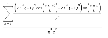
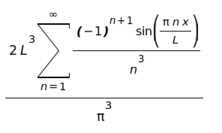
(%i15) mixed_wave(T(x,t),f(x),g(x),1,0,1,0,bb1(t),bb2(t),x,t,L,c,inf);
(%o15)

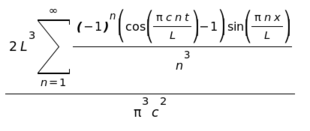
We can simplify the output a little bit:

(%i16) factor(%);
(%o16)

Mathematica™ (version 12.0) can not solve it, but Maple™ (version 2019) does. In case you want to compare the output given here with that of Maple™'s, please notice that

(%i17) fouriersin_series((a*L^2*x-a*x^3)/6,x,L,inf);
(%o17)

(%i18) kill(T,f,g,bb1,bb2)$

The Laplace equation

The 2D Laplace equation Δu=0 can be written either in Cartesian coordinates

Δu=u_xx+u_yy=0

or in polar ones

Δu=u_rr+¹⁄_r u_r+¹⁄_r² u_θθ=0

These can be used in conjunction with Dirichlet or Neumann conditions, on a variety of domains. Accordingly, pdefourier offers several commands: dirichlet_laplace_rectangle, neumann_laplace_rectangle, dirichlet_laplace_disk, neumann_laplace_disk, dirichlet_laplace_wedge, neumann_laplace_wedge, dirichlet_laplace_annulus, and neumann_laplace_annulus. We refer to the pdf documentation file for more details and examples of each case.

Example 3 The following is a Neumann problem for the Laplace equation on a wedge defined by 0<θ<π/2, 0<r<1:

Δu=0
u(r,0)=0=u(r,a)
u_r(θ,r)= cos(4θ)

The solution is readily found:

(%i19) ur(theta):= if (0<=theta and theta<=%pi/2) then cos(4*theta)$
(%i20) neumann_laplace_wedge(R,%pi/2,ur(theta),theta,inf);
(%o20) The sum is over ℕ-{2}

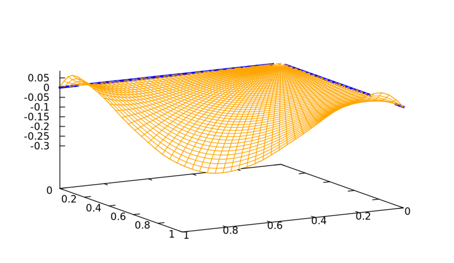
To get a graphical representation of the solution, we can truncate the resulting series:

(%i21) expr:neumann_laplace_wedge(1,%pi/2,ur(theta),theta,15)$
(%i22) u_r1:at(diff(expr,r),r=1)$
(%i23) draw3d(view=[67,151],surface_hide = true,
color = orange,
parametric_surface(r*cos(theta),r*sin(theta),expr,r,0,1,theta,0,%pi/2),
line_width = 3,
color = blue,
parametric(t,0,0,t,0,1),
color = blue,
parametric(0,t,0,t,0,1)
)$
(%t23)

Bessel functions

Maxima has built-in functions for computing values of the Bessel functions, but not of their zeros. These zeros are needed for solving some problems, notably the 2D wave equation on bounded domains. The package pdefourier implements a fast and efficient algorithm for this task, the command BesselJZeros calculates the zeros of Bessel functions of the first kind J_ν(x) when ν>-1. Thus, the 5th zero of J₄(x) is given by

(%i24) BesselJZeros(4,5);
(%o24) 20.82693295696241

while the first five zeros of J₄(x) are obtained using the optional argument `all`:

(%i25) BesselJZeros(4,5,all);
(%o25) [7.5883424345038,11.06470948850117,14.37253667161759,17.61596604980481,20.82693295696241]

There is no upper bound in the order (although precision decreases with higher values of ν). Many algorithms use some variant of MacMahon's formula or the Halley method, so they are not capable of working with big values. For instance, neither Mathematica(TM) nor Wolfram Alpha can compute this:

(%i26) BesselJZeros(146225,3);
(%o26) 146456.0070601201

The zeros of the derivatives of first-order Bessel functions can be computed with the aid of formulas such as

J'₀(z)=-J₁(z)
J'_ν(z)=(J_ν-1(z)-J_ν+1(z))/2

In this case, we have the command BesselJdiffZeros. For instance, the following table gives the first 5 zeros of J'_m(x) for 0≤m≤10, and is to be compared with the one in http://wwwal.kuicr.kyoto-u.ac.jp/www/accelerator/a4/besselroot.htmlx

(%i27) apply(matrix,makelist(BesselJdiffZeros(j,5,all),j,0,10));
(%o27)
[3.831705970207512,7.015586669815619,10.17346813506272, 13.32369193631421,16.47063005087759], [1.84118378134066,5.331442773525031,8.536316366346284,11.70600490259207,14.86358863390901], [3.05423692822714,6.706133194158456,9.96946782308759,13.17037085601612,16.34752231832178], [4.201188941210528,8.015236598375953,11.345924310743,14.58584828616704,17.78874786606648], [5.317553126083997,9.28239628524161,12.68190844263889,15.96410703773154,19.19602880004888], [6.41561637570024,10.51986087377231,13.98718863014031,17.31284248788464,20.57551452138685], [7.501266144684142,11.7349359530427,15.26818146109787,18.6374430096662,21.93171501780223], [8.577836489714077,12.93238623708957,16.52936588436695,19.94185336652735,23.26805292645757], [9.647421651997215,14.11551890789461,17.77401236691525,21.22906262285313,24.58719748631768], [10.71143397069994,15.28673766733295,19.00459353794605,22.50139872677729,25.89127727683913], [11.77087667495558,16.4478527484865,20.22303141268171,23.76071586032743,27.18202152719051]

As an application, consider the 2D wave equation (with c²=5):

u_tt=5(u_xx+u_yy)

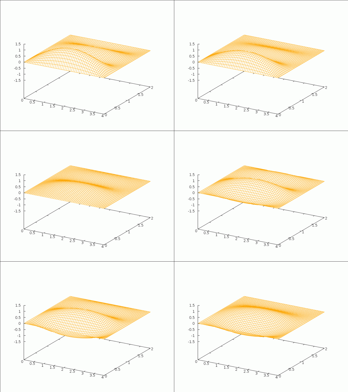
on the rectangle (x,y)∈[0,4]x[0,2], with intial configuration f(x,y)=x(4-x)y(2-y)/10 and vanishing initial distribution of velocities. We solve that problem and create an animation of the solution with the following commands:

(%i28) f(x,y):=x*(4-x)*y*(2-y)/10$
(%i29) g(x,y):=0$
(%i30) wave2d_rectangle(sqrt(5),4,2,f,g,4,4)$
(%i31) expr:%$
(%i32) wxanimate_draw3d(s,makelist(i/10,i,0,32), surface_hide=true,zrange=[-1.5,1.5], color=orange, parametric_surface(x,y,subst(t=s,expre),x,0,4,y,0,2) ),wxanimate_framerate=8$
(%t28)

Software used

Maxima - Maxima, a computer algebra system
wxMaxima - wxMaxima, a graphical front-end for Maxima

Authors

Emmanuel Roque Jiménez - emmanuelroque
José Antonio Vallejo Rodríguez - josanvallejo

License

This project is licensed under the GNU General Public License v3.0 - see the LICENSE.md file for details

Acknowledgments

Thanks to the Maxima's developers team, for maintaining such a wonderful software
Thanks to the KeTCindy team, particularly its main developer Setsuo Takato, for their support

caadxyz/pdefourier