Tensorflow demo code for paper Distributional Adversarial Networks by Chengtao Li*, David Alvarez-Melis*, Keyulu Xu, Stefanie Jegelka and Suvrit Sra.
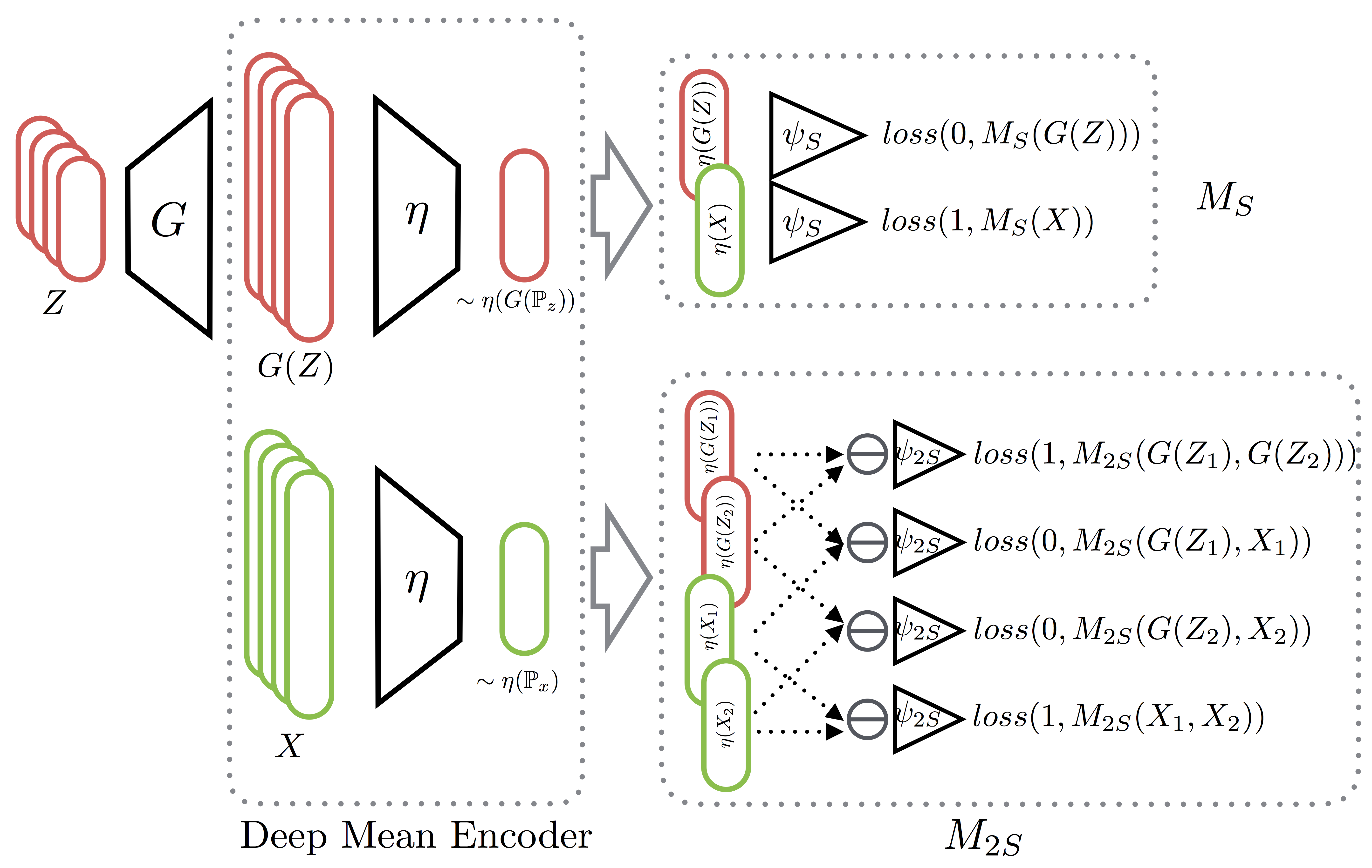
The main difference with the original GAN method is that the Discriminator is operates on samples (of n>1 examples) rather than a single sample point to discriminate between real and generated distributions. In the paper we propose two such type of methods:
- A single-sample classifier
$M_S$ which classifies samples as fake or real (i.e. a sample-based analogue to the original GAN classifier) - A two-sample discriminator
$M_{2S}$ which must decide whether two samples are drawn from the same distribution or not (reminiscent of two-sample tests in the the statistics literature)
Both of these methods relies on a first stage encoder (Deep Mean Encoder), which embeds and aggregates individual examples to obtain a fixed-size representation of the sample. These vectors are then used as inputs to the two types of classifiers.
A schematic representation of these two methods is:
Python 2.7tensorflow >= 1.0numpyscipymatplotlib
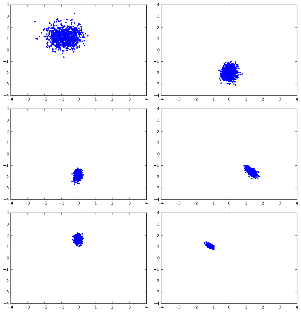
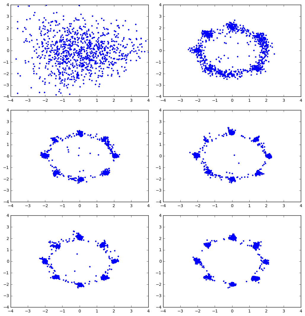
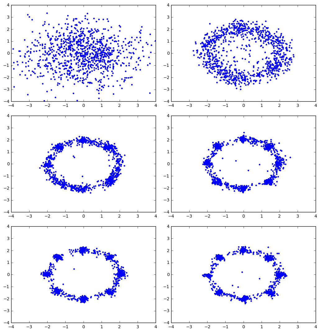
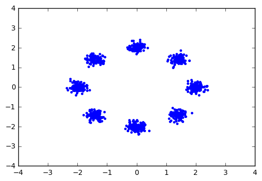
A self-contained implementation of the two DAN models applied to a simple 2D mixture of gaussians examples can be found in this notebook in toy folder. Some of the visualization tools were borrowed from here.
| Vanilla GAN | DAN-S |
|---|---|
 |
 |
| DAN-2S | Ground Truth |
|---|---|
 |
 |
This part of code lies in mnist folder and is built based on DCGAN Implementation.
To train the adversarial network, run
python main_mnist.py --model_mode [MODEL_MODE] --is_train True
Here MODEL_MODE can be one of gan (for vanilla GAN model), dan_s (for DAN-S) or dan_2s (for DAN-2S).
To evaluate how well the model recovers the mode frequencies, one need an accurate classifier on MNIST dataset as an approximate label indicator. The code for the classifier is in mnist_classifier.py and is adapted from Tensorflow-Examples. To train the classifier, run
python mnist_classifier.py
The classifier has an accuracy of ~97.6% on test set after 10 epochs and is stored in the folder mnist_cnn for later evaluation. To use the classifier to estimate the label frequencies of generated figures, run
python main_mnist.py --model_mode [MODEL_MODE] --is_train False
The result will be saved to the file specified by savepath. A random run gives the following results with different model_mode's.
| Vanilla GAN | DAN-S | DAN-2S | |
|---|---|---|---|
| Entropy (the higher the better) | 1.623 | 2.295 | 2.288 |
| TV Dist (the lower the better) | 0.461 | 0.047 | 0.061 |
| L2 Dist (the lower the better) | 0.183 | 0.001 | 0.003 |
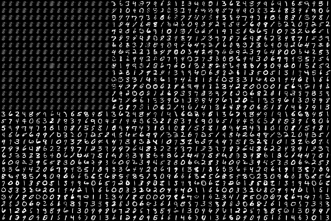
The following visualization shows how the randomly generated figures evolve through 100 epochs with different models. While for vanilla GAN the figures mostly concentrate on ''easy-to-generate'' modes like 1, models within DAN framework generate figures that have better coverages over different modes.
| Vanilla GAN | DAN-S | DAN-2S |
|---|---|---|
 |
 |
 |
If you use this code for your research, please cite our paper:
@article{li2017distributional,
  title={Distributional Adversarial Networks},
  author={Chengtao Li, David Alvarez-Melis, Keyulu Xu, Stefanie Jegelka, Suvrit Sra},
  journal={arXiv preprint arXiv:1706.09549},
  year={2017}
}
Please email to ctli@mit.edu should you have any questions, comments or suggestions.
