library(cedwards)
library(ggplot2)
#> Warning: package 'ggplot2' was built under R version 4.2.2

cedwards

The goal of cedwards is to formalize the functions I store as gists or keep adding as new functions for every new project. These are include organization functions (skeleton_maker.R), plotting convenience functions (gfig_saver.R), and some other misc functions. This is a living package, and will continue to grow as I aggregate my common tools.

Installation

You can install the development version of cedwards from GitHub with:

# install.packages("devtools")
devtools::install_github("cbedwards/cedwards")

Todo

List of some additional functions I will add as time permits.

FunPlotter

Sometimes we need quick prototypes for a given function. Especially common when talking about distributions in stats classes. FunPlotter should take the desired functional form (in tex form? in R form? something else?) and, optionally, x and y limits, and create a reasonable visual of the function. Bonus points if it can optionally take the function and a list (LIST) of parameters, where if 1 or 2 of the parameters are provided as vectors, the resulting figure uses geom_path and / or facet_wrap to capture the variation.

BootMuffler

Apply the Muff et al. 2021 treatment to bootstrapped results using confidence intervals. Goal is to return the 95% CI (for reporting, potential plotting), 84% CI (for potential plotting), and either “no evidence”, “weak evidence”, “moderate evidence”, or “strong evidence” based on the 99%, 95%, 90% CLs. Should also (optionally?) provide the citations for Muff et al, and for Payton et al. 2003 (which is the citation for using 84% CIs for plotting.

Usage

Communication

When giving talks or lecturing, I often want to make a series of related plots, each with additional information on them. For example, I might show a functional form, then simulated data based on that functional form, then a model fitted to the simulated data. ggplot_lister() and ggplot_list_saver() streamline the workflow for this process by allowing you to specify a list of ggplot layers interspersed with commands to “save” the layers up to a given point, or remove previous layers before continuing.

Organization

Project structure

For setting up new projects, I’ve settled on a consistent file directory structure, and I find it is helpful to prepopulate a list of recommended reviewers and some other documentation files. This is streamlined in skeleton_maker(), which generates a new project with location specified by filepath.

Replicable figures

A common issue (for me anyways) is that it’s easy to have scripts saving figures, then come back later and

not remember the details on that figure (what parameters was I using?),
not remember which script generated it (I actually wrote some CLI code to search all R files for instances of the file name, but for auto-generation of figures based on parameter or scenario names, sometimes the full file name isn’t listed in a single sequence in thes cript), and
realize I need to tweak a few pieces, but be unable to do so unless I track down, tweak, and re-run the script that generated the figure.

My solution is gfig_saver. This is largely a wrapper for ggsave(), but adds some functionality. First, it saves the figure in both .jpg and .pdf formats - depending on usage, one or the other format is handier, and it stinks to have to regnerate things. Second, it explicitly requires a description in string / vector of string form, which can take the form of a prototype figure caption. This is saved as a metadata file with the same naming structure as the figures, and can include information about what script generated the figure and when it was made. I highly encourage you (and myself) to take advantage of this. In the long run, I would have saved a lot of time by better documenting where figures came from. Finally, the function also saves the ggplot object as .RDS file. You can then load that into an R script and tweak themes, add or remove layers, etc, without having to re-run the original script. Obviously it’s good practice to keep your original script updated, but this can be a huge time saver for something like tweaking formatting settings when submitting for publication in a new journal.

Convenience

`cd()`

This is a wrapper for setwd() that lets you change directories using the linux command name.

`doy_2md()`

Working with phenology (the timing of life history events in ecology) often means calculating the day of year of some process. But finding that the mean day-of-year of activity for the Monarch butterfly is day 134 is hard for many of us to parse (unless we’ve been working in phenology for a long time, like collaborators Cheryl Schultz or Elizabeth Crone). Is that number reasonable? What’s the actual date? doy_2md to the rescue!

doy_2md(134)
#> [1] "May 14"

This function can also take vectors, and can be useful if you want to specify arbitrary ticks on a plot (although the lubridate package can be helpful with this). Here’s an example without clear labels:

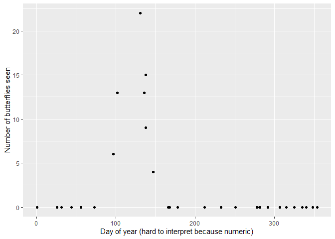
## make up some data to plot
N = 30
dat = data.frame(doy = round(runif(N)*365))
dat$count = rpois(N, lambda = 1000*dnorm(dat$doy, mean = 120, sd = 12))
ggplot(data = dat, aes(x = doy, y = count))+
  geom_point()+
  xlab("Day of year (hard to interpret because numeric)")+
  ylab("Number of butterflies seen")

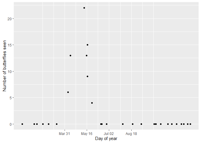
And now, using doy_2md to help with tick marks:

ticks.df = data.frame(breaks = seq(90, 230, length = 4))
ticks.df$label = doy_2md(ticks.df$breaks, short=T)
ggplot(data = dat, aes(x = doy, y = count))+
  geom_point()+
  xlab("Day of year")+
  ylab("Number of butterflies seen")+
  scale_x_continuous(breaks = ticks.df$breaks,
                     labels = ticks.df$label)